How & When To Create A Data Model [5 Simple Steps]

Excel data models are made to help users integrate data from multiple tables.

It is of great use to professional Excel users as it saves tons of effort and time that otherwise goes into collating data manually.

All that you need to know about creating a data model in Excel is pulled together in the article below.

Data models are very common in todays workplace. Delegates on our Excel Courses ask about them every week!

What Is A Data Model?

The Data Model feature of Excel is specifically designed to help users collate data scattered across multiple data tables.

Under data models, two or more tables are transformed into one based on one or more common columns.

Using data modeling, you can bring together data from multiple tables or external sources on the platform.

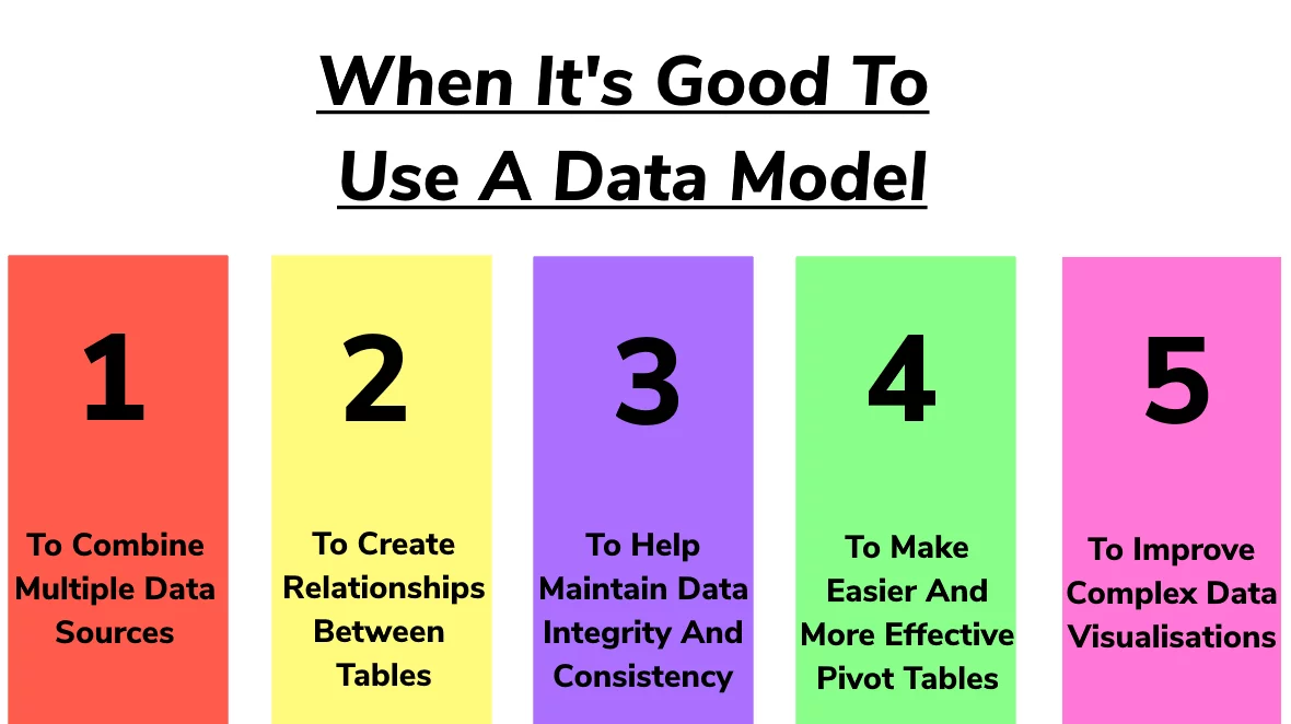
A data model offers a wide variety of advantages to Excel users, some of which are as follows.

1. They  enable Excel users to create Pivot Tables with sheer ease.
2. As it helps integrate tables, it is a useful tool when it comes to data analysis using Power View in Excel.
3. It enables the export of data from different external data sources.
4. It is a great substitute for the complicated VLOOKUP function of Excel.

Having all your data in one place will not only help your efficiency, but show your supervisor you know how to keep multiple spreadsheets under control.

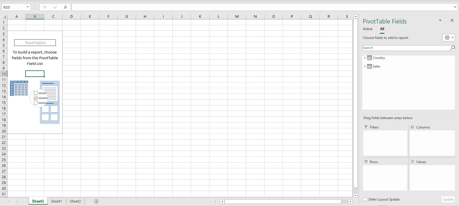
How To Make A Data Model

To learn how to create a data model in Excel, let’s quickly stipulate an example.

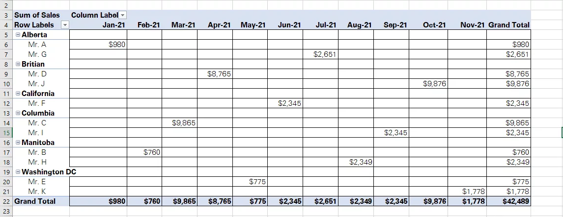
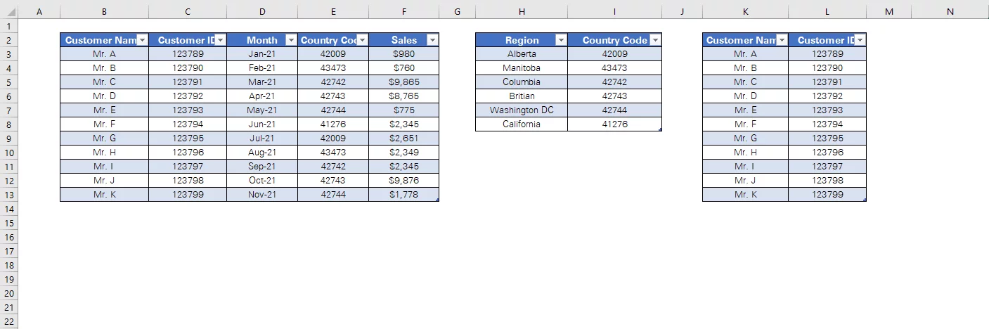
Below is a screenshot that shows the sales data of a Company.

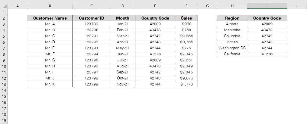
However, the main table only includes the country code which is of little use until the parallel Region against each code is mentioned against each sale.

The information of the corresponding region against each country code is available in the parallel table.

To combine them both in a Data Model, here are the steps to be followed.

Step 1:

First, take note of the type of data. The data related to sales is simply populated in an Excel file.

However, as data modeling integrates data tables, it is important to ensure that the source data is in the form of data tables.

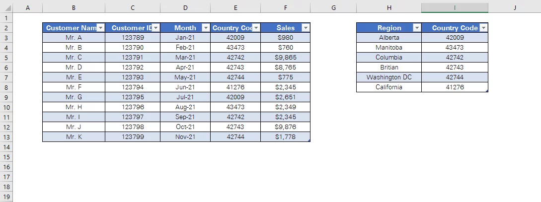
To do so, select each dataset (Including headers) and turn it into a data table as follows.

Insert > Table

Once this is done, here is what the data tables should look like.

Step 2:

Next, name each table for ease of building connections.

Select each table > Tools > Table Name

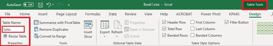
Once this is done, all your tables would be uniquely named.

We have named the first table as ‘Sales’ and the other as ‘Country’ depending upon the information contained therein.

Step 3:

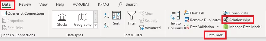
Next, you need to build a relationship between both tables through the following route.

Data > Relationships

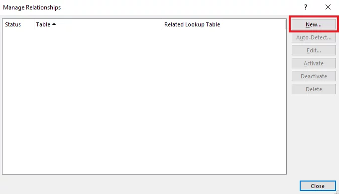
This opens up the ‘Manage Relationships’ dialogue box as follows.

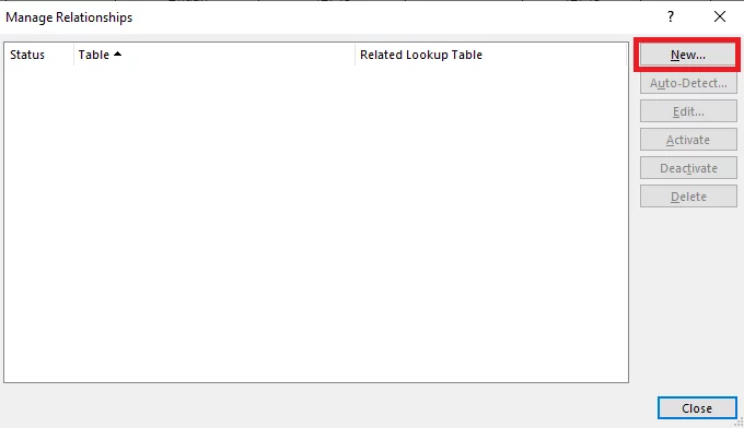
Click on ‘New’ as shown above to form a relationship between both the data tables.

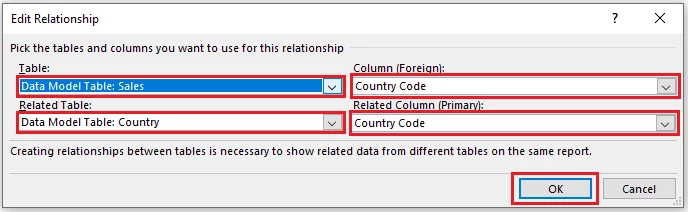
This takes you to the ‘Edit Relationship’ dialogue box.

To relate both the Table and the Related Table, select the column common between both.

As we have the Country Code common to both, we have selected the same as the Column (Foreign) and the Related Column (Primary).

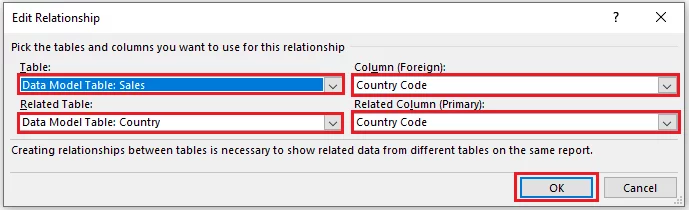
This forms a relationship between both tables.

See more details of building relationships in Excel in the segment that follows.

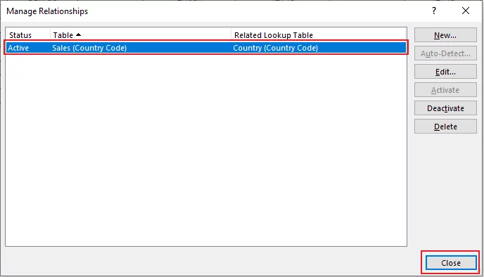
Once the relationship is formed, it appears under ‘Manage Relationships’ as follows.

Step 4:

Next, create a pivot table by simply launching the editor as follows.

Insert > Tables > Pivot Table

This opens up the Create PivotTable dialogue box as follows.

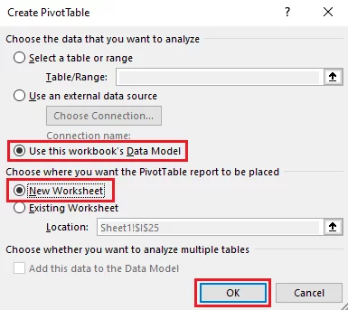
As we have already built relations among the data tables, a data model is formed in Excel memory.

Simple select the option ‘Use this workbook’s Data Model’ and the destined location as highlighted above.

Step 5:

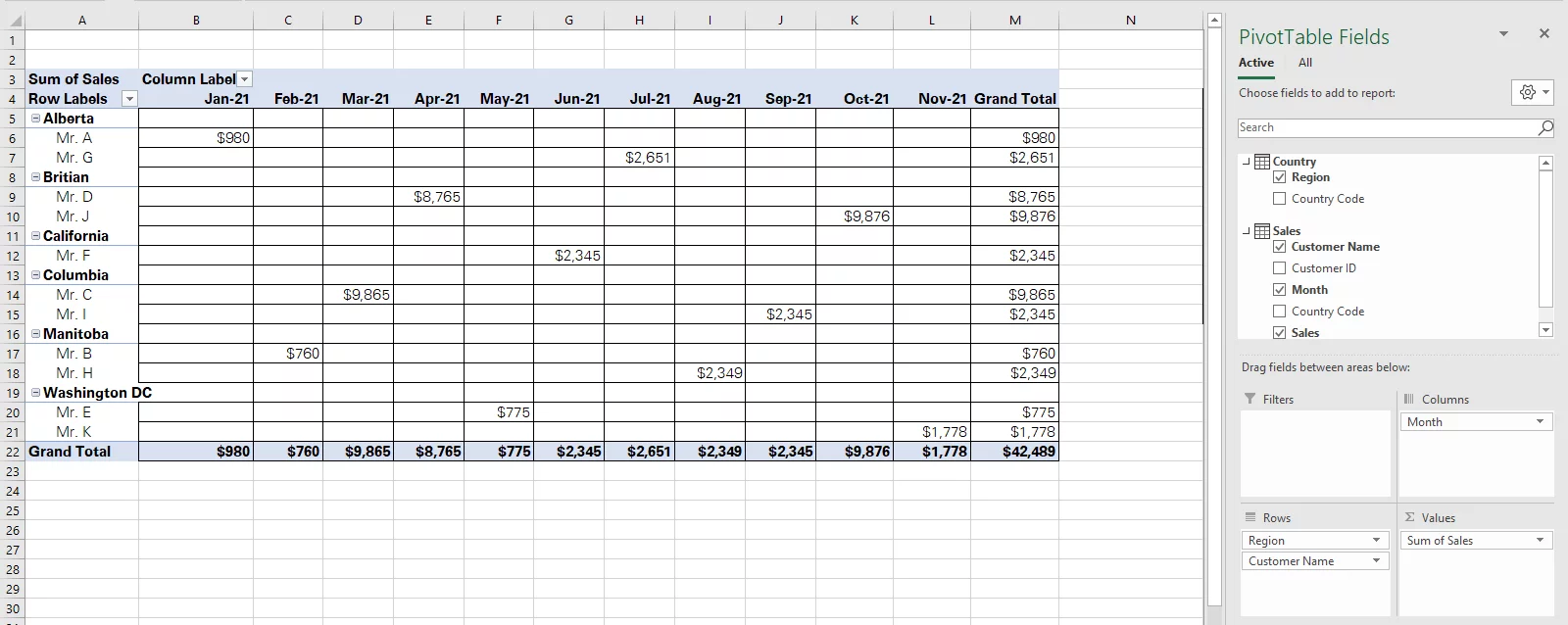
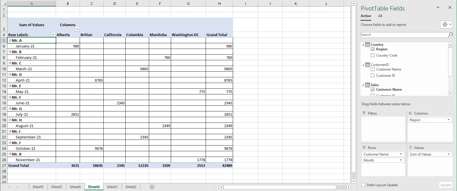
Both the tables now appear under the Pivot Table fields.

To categorize the sales made to each customer in terms of country of sale along with the sum of sales achieved each month, expand each table by clicking on it.

Drag the column ‘Region’ and ‘Customer Name’ to Rows.

Similarly, take ‘Months’ under the box Column and ‘Sales’ to the Values box to have the month-wise sales populated against each region and customer.

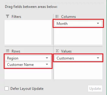
Here are how the final results look after all the necessary formatting.

Learn more Excel data analysis techniques here.

Data Model Use Cases

Data Models, being one of the most advanced functions of Excel, are of great use to both regular and proficient Excel users.

Here are a few practical cases where you may readily employ them.

• Globally spread businesses often prepare individual accounts for each region.
  • These accounts are then consolidated together to prepare the summary financials for the entire business.
  • A data model can be conveniently used to consolidate these accounts.
• If you prepare your domestic budgets using Excel and have all your monthly bills scattered across different files:
  • You can bring them along in a single table using a data model.

In addition to the foregoing, a data model can surprisingly help you with your routine data analytics.

Especially for businesses who use Excel for accounting and bookkeeping, data modeling is their go-to tool.

Creating Relationships

Creating relationships between tables turns out to be a tricky step of the data modeling exercise.

However, it only requires you to understand how things work at the Excel end.

While creating relationships, you will come across four options, each of which is explained below.

• Table: This refers to the table that contains the main data to be linked with other data in Excel.
• Column (Foreign): This refers to the column in the above table where the values are to be looked up.
• Related Table: This refers to the table where the values are to be looked up for.
• Related Column (Primary): This refers to the column in the related table that is common to the main table.

Excel links both the tables based on these two, foreign and primary columns.

Let’s create multiple relationships through the example below to see how the linking works.

Below is a data set that contains multiple tables relevant to the sales of a Company.

To create relationships among them all, here are the steps to be followed.

Step 1:

First of all, ensure all the tables of your data set are constructed as a ‘Table’ in Excel.

If not, Excel won’t recognize them as tables when creating relationships.

You can quickly turn your dataset into a table by going to Insert > Table.

Next, name each table for ease of reference. We have named all the three tables as Sales, Country, and Customer ID, respectively.

Step 2:

Go to Data > Data Tools > Relationships.

Pro Tip: If the ‘Relationships’ option of your data tab is greyed out (frozen for selection), probably your Excel sheet consists of only a single table.

Must note that while creating relationships, Excel considers tables of all the Excel books launched at any given time and not a single book.

From the ‘Manage Relationships’ window, select ‘New’ as shown below.

 

This opens up the ‘Edit Relationship’ window.

Now, to create a relationship between the first two tables i.e. Sales and Country, let’s start choosing the options.

Under the option Table, select ‘Sales’ and under the option Related Tables, select the option ‘Country’.

Now to link both these tables, select the column that is common to both the tables under the option Column (Foreign) and Related Column (Primary).

This is how it should look like when populated.

Click ‘Okay’, and Excel would construe it as a relationship.

Note: The Related Table (Country) where the value is to be looked up contains unique values i.e. no region is repeated.

However, the same country code appears for more than once in the main table (Sales). For example, 42009 appears at Serial No. 1 and Serial No. 7.

The Related table must only contain unique values. Such relations are known as one-to-many relationships.

Looking for more Excel tips? Read our guide on how to Recover Unsaved Files in Excel here!

Step 3:

Do the same to build a relationship with the last table.

Open the ‘Edit relationship’ window and select Sales as the Table, and Customer ID as the Related Table.

Next, under the foreign and primary column options select the column that is common to both i.e. Customer ID.

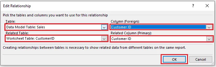
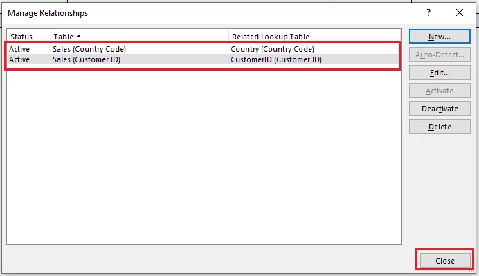
Hit ‘Okay’, and there you have your relationships created.

You can view the relationships created in Excel under the ‘Manage Relationships’ window as follows.

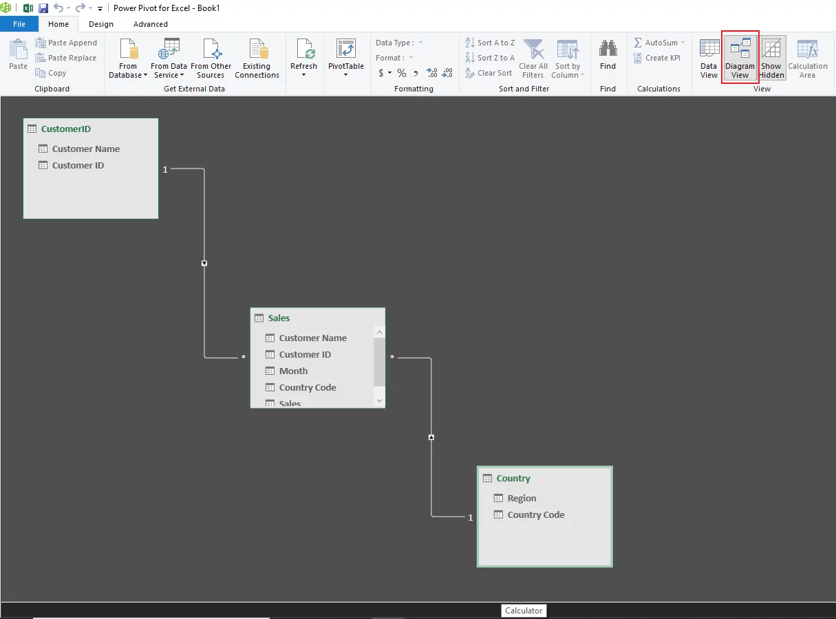
Power Pivot Diagram View:

Also, once you have created relationships, you can go over them through Power Pivot Diagram.

You may access Power Pivot Diagram through the following route.

Data > Data Tools > Manage Data Model

Within the window that opens up, select ‘Diagram View’ from ‘View’ in the Home Tab as highlighted below.

This shows a diagram view of the relationship you have created.

Pro Tip: If the ‘Manage Data Model’ option is greyed out, you probably don’t have it enabled, or your Excel version is not supportive of it.

You can enable the Data Analysis add-in once prompted after you click on the said option.

For more on Excel Functions, read our guide here on the XMATCH Function!

Add Data To Your Data Model

After we have come across the tricky exercise of putting together models in an Excel sheet, what if some datasets are still left out?

For Excel users who employ models, it is often the case.

At times, this is an indispensable part of the data collation phase as the underlying data may undergo regular updates.

Or even otherwise, you may forget to add a chunk of data (a table or two) to your final data model.

In either case, embedding additional data into your data model is easier than you think.

This can be primarily done as follows.

If you’ve already constructed your Pivot Tables, simply add data to the excel data model.

Or, you may quickly set up a Pivot table using the existing data model tables and then add additional data to it.

However, the following chunk of data needs to be incorporated in the foregoing data model too.

Step 1:

Convert the data that you want to be added to the data model in a table. Simply select it and turn it into a table as follows.

Insert > Table

Step 2:

Select this table (or a cell from this table) and go as follows.

Data > Get & Transform Data > From Table / Range

Step 3:

Within the home tab of Power Query Editor, select the option ‘Close and Load’ as appears on the left side of the panel.

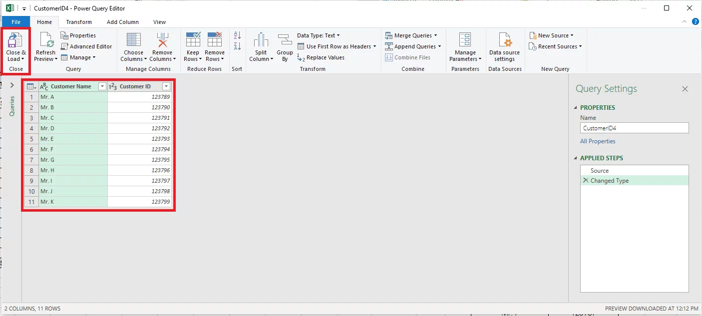
Step 4:

This opens up the ‘Import Data’ dialogue box as follows.

 

 

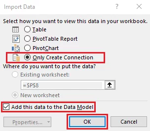
As shown in the image above, select how you want the data to be viewed in the Workbook.

As we only want to embed the data into the data model, select ‘Only Create Connection’.

For the location of the data, select ‘Add this data to the Data Model’.

And that’s it – you have your data added to your data model.

It should now appear as a field under the PivotTable fields.

You can expand it to incorporate it in your Pivot Table as required.

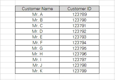
We have added the Customer ID along with the name of each customer in our Pivot Table as shown below.

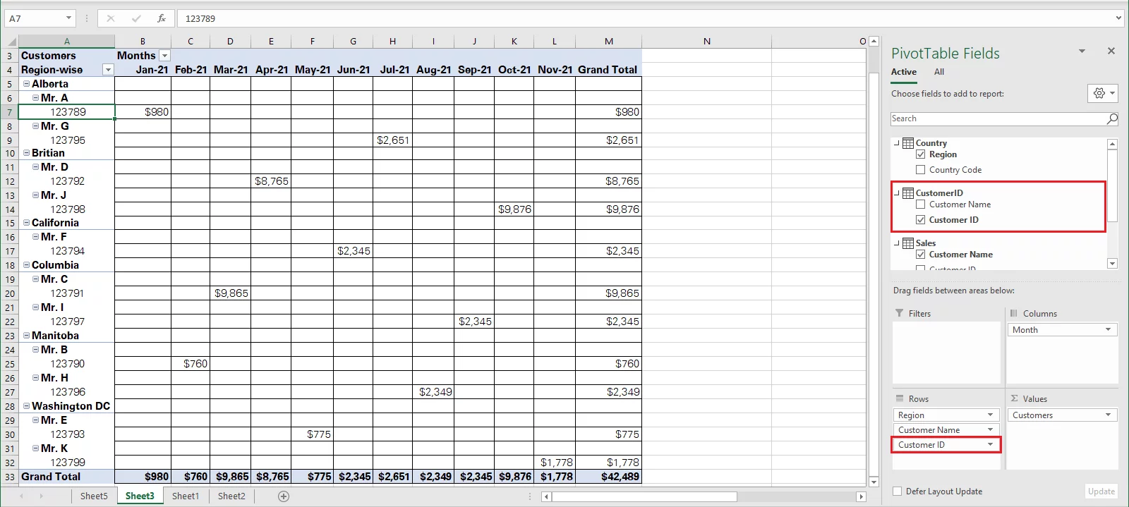
Pro Tip: What if you don’t want to add a whole new table to the Pivot Table but only a new column or row?

Simply make the desired changes to the source data (the tables included in the Pivot Table) and go to Data > Refresh > Refresh All.

Making A Pivot Table

Forming Pivot Tables from a data model is a short process with a few thoughtful clicks, and you are all done.

Take a look at the example below to see how you can quickly assemble a Pivot Table out of a Data Model.

Using the same data as above, we have three tables; each containing different information relevant to the sales of a Company.

To convert multiple tables into a Pivot Table, you first need to put them together as a Data Model.

To do so, let’s start creating relationships between them.

As is evident, the common column between the first two tables, i.e. Sales and Country is Country Code.

Whereas, the common column between the table Sales and CustomerID is, Customer ID.

Using the same information, we have built relationships as follows.

Next, launch the Power Pivot Table as follows.

Insert > Tables > PivotTable

This launches the ‘Import Data’ dialogue box.

As we’ve already created a data model by creating relationships among tables, check the Option ‘Use this workbook’s data model’.

Also, select the destination where you want the Pivot Table to be located, be it in the same worksheet or a new one.

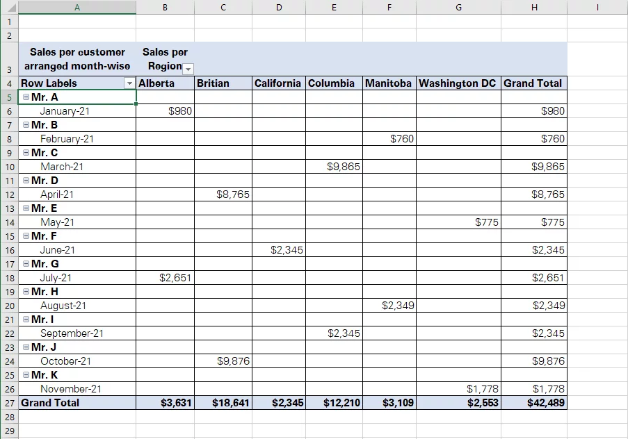
Hit ‘Okay’ and Excel would form a Pivot Table. Next, drag and drop the Power Pivot fields to rows, columns, values, and filters to have your Pivot Table presented to your choice.

Take a look into the fields column to see how each table appears there by the name designated to it. Click on it to expand it column-wise as shown below.

Format the sales amount as currency, add some borders and brush the final look to have a month-wise sale report of each region ready.

There’s much more to Power Query that you may want to learn.

Conclusion

At a glance, data modeling in Excel might seem like adding unnecessary chores to your plate.

However, that is only in case you have a simple set of data whereby VLOOKUP might act as a time-saver.

As the data grows in magnitude, you’d vouch for data modeling as it helps collate data efficiently and effortlessly.

Try practicing using different datasets to master the technique of simplifying data, no matter how extensive.

Looking for more top tips on Excel? Read our guide here to Creating a Flowchart in Excel or our article about creating a histogram.