
XMATCH Functions – Master Excels Array Tools!
Contents
Most people using Excel, have used the MATCH function.
However, with more features and flexibility, the XMATCH function is much more powerful.
It helps you look out for values and identify their position from a given range or array.
Learn all about how to use this clever function in the article below or on one of our City of London Excel training!
Excel XMATCH Function
The Excel XMATCH function from the dynamic array tools of Excel is an advanced version of the MATCH function.
It enables users to find the relative position of a specific data entry within an array or range.
It not only offers more features than the MATCH function but is also flexible and easier to use.
Syntax
Syntax of the XMATCH function looks as below.
=XMATCH (lookup_value, lookup_array, [match_mode], [search_mode])
Arguments
It’s time we break down the arguments posed by the syntax of the XMTACH function to decipher it better.
- Lookup_Value – As the name verily tells, this argument specifies the value to be looked up for.
- Lookup_Array – This argument specifies the range or array where the lookup value is to be searched for.
- Match_Mode – This is an optional argument. It specifies the type of value to be looked for.
Users may specify either of the following four arguments as the match mode.
| Arguments | Match Mode |
| 0 | Exact Match |
| -1 | Exact match or the next smaller value |
| 1 | Exact match or next larger value |
| 2 | Wildcard match |
| If Omitted | Set to 0 by default |
- Search_Mode – This is an optional argument. It specifies starting from where the search for the lookup value is to be performed.
Users may specify either of the following four arguments as the search mode.
| Arguments | Search Mode |
| 1 | Search from the first value |
| -1 | Search from the last value |
| 2 | Binary Search Ascending |
| -2 | Binary Search Descending |
| If Omitted | Set to 1 by default |
Return Value
XMATCH function returns the relative position of the specified value from the lookup array. The return value is numeric.
Functions Library
Find out the XMATCH function from the Functions Library as follows.
Formulas > Functions Library > Lookup & Reference > XMATCH
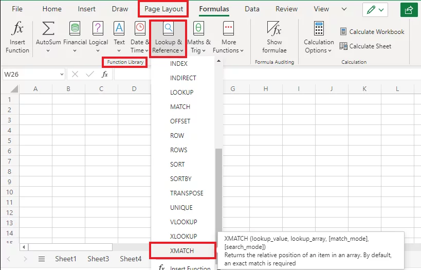
Note: The XMATCH function is only available to the subscribers of Microsoft 365 for Excel 2019 and above versions.
Why would someone want to use it?
The XMATCH function of Excel is one of the most commonly used dynamic array tools of Excel in the financial modeling industry.
Not only that, it is the go-to tool for statisticians, forensic auditors, and many other data technicians.
For instance, as a money operator, you may want to instantly search all those currencies that equate to $0.5 from a list of hundreds of currencies.
Do not just go searching all the way manually.
Set up the XMATCH function to readily identify the relative position of each currency entry that meets the said criterion.
Luckily, Excel makes currency conversion very easy too!
XMATCH Use Cases
XMATCH function helps many Excel users from different fields of life. It can be of great help to professionals like statisticians, data analysts, researchers, and financial data modelers.
Even if you take it to domestics and regular day usage, the XMATCH function can help you ace a variety of tasks from your daily life.
The XMATCH function can be used by result compilers to know the number of students who gained a specific percentage or marks.
Specifying different match modes, you can search for students who gained immediately lesser or higher marks than a specific threshold.
It can be used by auditors to readily identify where an invoice is entered in a data set of invoices.
Businesses can use it to sort particular customer records from their sales data by specifying the name or ID of a customer as the lookup value.
As it helps look up for a value, the XMATCH function can be of endless use to different groups of people.
Using XMATCH to search for a specific item in an array – Basic Example
Apart from all the theoretical discussion, it’s time we stipulate a simple example to see the XMATCH function work.
The image below manifests the result sheet of XYZ School for the academic year 2021.
It contains the result of many students arranged position-wise.
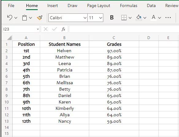
If you want to find the position of a particular student, say Aliya, how can you do it using the XMATCH function?
Step 1:
Activate the cell where you want the position of Aliya to be populated and compose the XMATCH formula as follows.
=XMATCH (“Aliya”, B2:B13)
- The first argument is the value that needs to be looked up from the array. It must be enclosed in double quotation marks.
- The second argument is the array where the value needs to be looked up. As the names are specified under column B (cells B2 to B13), we have specified it as the lookup array.
- The third and fourth arguments, being optional are omitted. Excel sets them to the default values of 0 and 1 respectively.
- This means the match_mode is set to 0 where Excel would only lookup for the exact match. And the search_mode is set to 1 where Excel would start searching from the first value. As the students are already arranged position-wise, and we want to find the relative position of Aliya, both the arguments fit our needs.
Step 2:
Hit ‘Enter’ to see the results as follows.
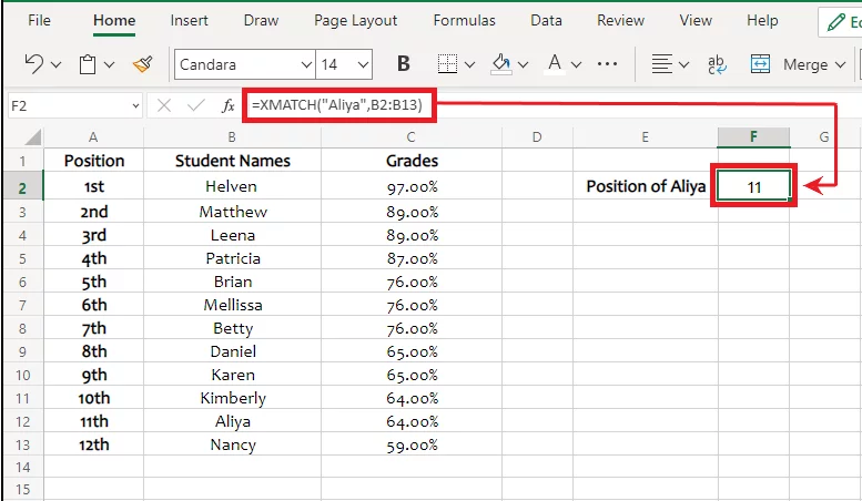
In the data, Aliya stands at the 11th position, and Excel has identified the same.
Pro Tip: As we have left the ‘Match Mode’ vacant, Excel has set it to ‘0’ by default.
That being said, Excel would only lookout for the exact spelling of ‘Aliya’.
If the spelling is not the same, the results put out by Excel will be as follows.
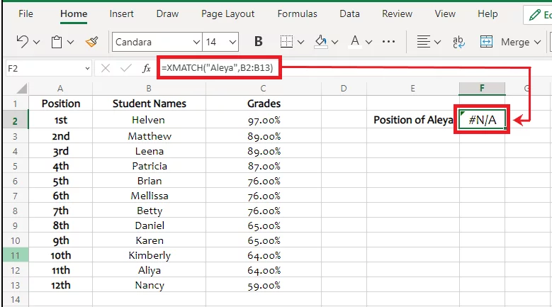
If you want to get rid of the exact match hunt of Excel, specify the third argument as 1 or -1 where Excel would lookout for the closest match if not the exact match.
More Examples
1. The XMATCH function with different search modes
The last argument from the XMTACH function i.e. the search mode is often misunderstood. To understand how this argument works, follow the example below.
The data below represents the details of the yearly ‘Best Employee’ title won by different employees of a Company over 10 years.
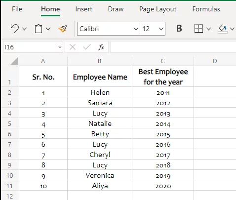
A closer look into the data reveals that the said title was won by the same employee multiple times. To know the first time when Lucy on the title, we can use the XMATCH function as follows.
Step 1:
Activate the cell where you want the results to be populated and compose the XMTACH function as below.
=XMATCH (“Lucy”, B2:B11,,1)
- The first argument is specified as “Lucy” enclosed in double quotation marks as it is the value to be looked up for.
- The second argument defines the lookup array where the value is to be looked up for i.e. B2:B12.
- The third argument is omitted and is assumed to be 0 by Excel by default. It is important to note that a comma is added before and after the vacant third argument before moving on to the fourth.
- The fourth argument is set to 1 as we want Excel to find and return the first year when Lucy won the award. Doing so, Excel will look up the specified array starting from the first value.
Step 2:
Hit ‘Enter’ to see results as follows.
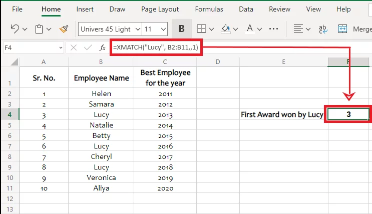
Excel returns the value 3 i.e. the first relative position of Lucy from the underlying data. The first time Lucy won the Best Employee Award was in 2013.
Although Lucy appears more than once in the given data, the other instances are not considered by Excel.
Let’s do it the other way around now.
Step 1:
Continuing with the same example as above, if we now want Excel to only identify the last time when Lucy won the best employee award.
To do so, compose the XMATCH formula as follows.
Activate the cell where you want the results to be populated and compose the XMTACH function as below.
=XMATCH (“Lucy”, B2:B11,,-1)
- The first argument is specified as “Lucy” enclosed in double quotation marks as it is value to be looked up for.
- The second argument defines the lookup array where the value is to be looked up for i.e. B2:B12.
- The third argument is omitted and is assumed to be 0 by Excel by default. We have added a comma before and after the vacant third argument before moving on to the fourth.
- The fourth argument is set to -1 as we want Excel to find and return the last year when Lucy won the award. Doing so, Excel will look up the specified array starting from the last value.
Step 2:
Hit ‘Enter’ to see results as follows.
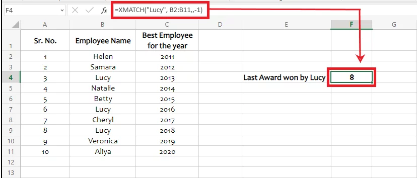
Excel returns the value 8 i.e. the last relative position of Lucy from the underlying data.
The last time when Lucy won the best employee award was in 2018.
Although Lucy appears more than once in the given data, the other instances are not considered by Excel.
2. XMATCH function with Wildcard characters
XMATCH function can be used with wildcard characters to look up different values.
There are two wildcard characters that you can employ in the XMATCH function.
- ? – A question mark equates to any value in the same order
- * – An asterisk equates to any sequence of characters
For example, from the list of continents below, we want to find the relative position of North America. It may be listed as North America or Northern America.
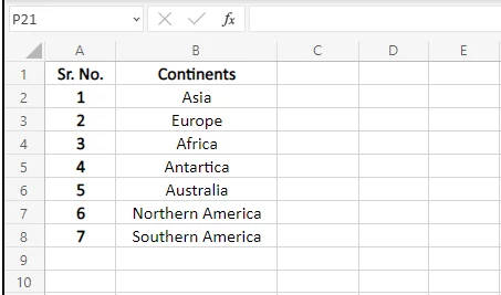
Not knowing the exact spelling used in the list, how can we specify the lookup value? This can be done using wildcard characters.
Step 1:
Activate the cell where you want the results to be populated and compose the XMATCH formula as follows.
= XMATCH (“North*”, B2:B8, 2)
- To specify the lookup value, we have used the wildcard character asterisk (*). This is because ‘Northern’ consists of three letters after the word ‘North’. Asterisk equates to any number of letters in any sequence after the word North.
- The lookup array is defined as B2:B8 as it contains the names of the continents from where the look up value is to be looked up.
- The match mode is set to 2 i.e. wildcard character match.
- The fourth argument is left vacant so Excel will set it to 1 by default.
Step 2:
Hit Enter to yield results as follows.
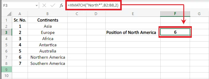
Excel finds the position of the word that contains ‘North’ and is most closely related to the specified criterion.
3. Nesting the XMATCH function into the INDEX function:
The XMATCH function is commonly used in pair with the Excel INDEX function as follows.
This is for the reason that, at times, we not only want to find the relative position of a specific value but the value itself.
The INDEX function serves the said job. For instance, the data in the example below states the ages of multiple people.
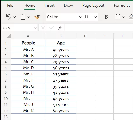
From this data, if you instantly want your hands on the age of Mr. D, how can you do that?
It is hectic to go back looking into the data for the entry of Mr. D and then copying his age from there to the destined location.
To your good, this can be done through a single formula using the XMATCH and INDEX functions together as devised below.
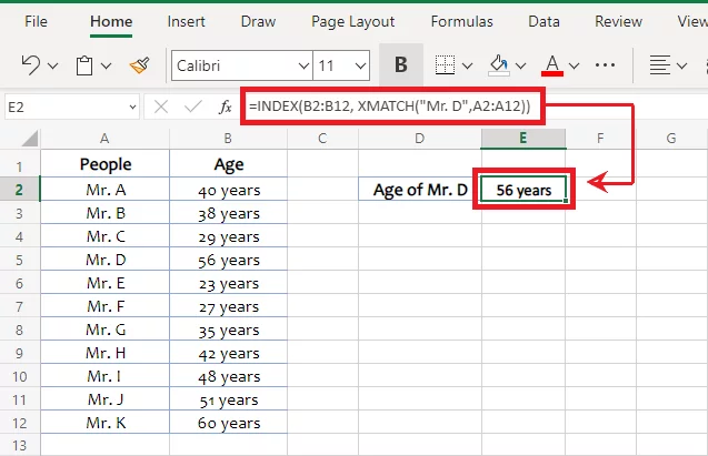
Step 1:
The first step is to put together the XMATCH formula. We want Mr. D (the lookup_value) to be looked up from the column of names A2:A11 (the lookup_array).
The formula would thus, be put up as follows.
=XMATCH (“Mr. D”, A2:A11)
This formula would return the relative position of Mr. D from the said column as a numeric value.
Step 2:
The next step is to set up the INDEX function by nesting in the XMATCH function as follows.
= INDEX (B2:B11, XMATCH (“Mr. D”, A2:A11))
- The first argument of the index function specifies the range from where the value is to be sought and returned.
- The second argument specifies the row wherefrom the value is to be returned. In place of the second argument, we have incorporated the XMATCH function; the product whereof would be the relative row number of Mr. D’s entry.
- The third and fourth arguments of the INDEX function are optional and are omitted.
Step 3:
Press ‘Enter’ to see Excel pick out Mr. D’s age for you in the designated cell as follows.
You can also nest the SORT and SORTBY dynamic array functions to pre sort the data!
XMATCH Troubleshooting
Following are some of the common problems experienced by Excel users when working with the XMTACH function.
1. Case insensitivity
The Excel XMATCH function, by default, is case insensitive. That means if a cell within your data contains the value ‘FedEx’, you can specify the lookup value as ‘fedex’ or ‘Fedex’ or ‘FEDEx’ or any combination of capital and small cases.
The XMATCH function would spot it out from the source data even if the case is inconsistent.
However, it is at times that we need to make a case-sensitive search. To do that, you can nest the EXACT function into the XMATCH function.
2. Inappropriate Match Mode
Most of the XMATCH function problems of Excel users originate from their inability to decipher the right match mode that meets their needs.
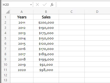
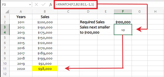
For the data above, if you want to know the relative position of all those years where the sales were equal to or close to $100,000, the XMATCH formula may be set in two ways.
=XMATCH (F2, B2:B11, -1,1)
In the formula above, as we have specified the match mode as ‘-1’, Excel would find the exact or next smaller value to $100,000.
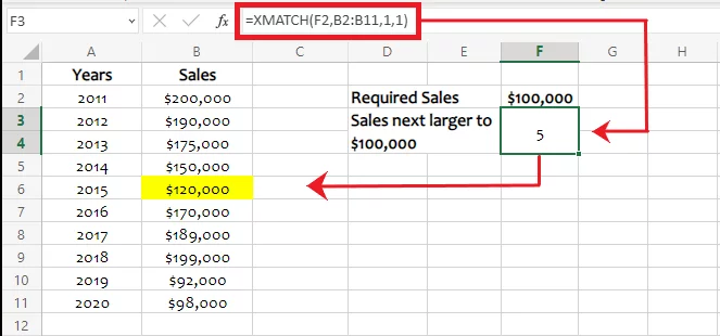
The formula above may also be set up as below.
=XMATCH (F2, B2:B11, 1,1)
In the formula above, as we have specified the match mode as ‘1’, Excel would find the exact or the next larger value to $100,000 from the lookup array.
If you’re keen to learn more amazing functions, check out the SEQUENCE dynamic array tool next.
Conclusion
The dynamic array tool of XMATCH can be of help for many Excel users from different rounds of life.
Practice a few examples from above to master it in no time.
We also have a complete guide on Excel array formulas for a more comprehensive look at arrays.


- Facebook: https://www.facebook.com/profile.php?id=100066814899655
- X (Twitter): https://twitter.com/AcuityTraining
- LinkedIn: https://www.linkedin.com/company/acuity-training/