Introduction to Slicers in Excel

Slicers in Excel are often used together with Excel tables and Pivot tables.

What are they used for? Quick filtering of data from huge, densely packed data sets. What distinguishes Slicers from ordinary data filters is their visual appeal and ease to use.

The article below covers all details about Slicers in Excel – how to create them, use them, format them and how to tackle potential issues they might pose.

Stay tuned until the end to cover them all.

What Are Slicers In Excel?

Have you seen these interactive menus in Excel? Where you choose an option, and the Excel sheet reacts accordingly.

These are Excel slicers. You may make them for an Excel table or a Pivot table. In short, for any data set where filters are to be used, you may insert slicers.

As they are graphic and interactive, they go very well with Excel dashboards. However, you may also use them for ordinary data tables in Excel.

They are easy to insert and use. Best part, they make your work a lot more presentable.

Learning how to make your worksheets presentable is a great way to impress your colleagues and supervisors!

This tutorial shows how you can add slicers to Excel for a given data table or pivot table. Not only that but also how you can customize it to your good.

Slicer Use Cases:

Excel Slicers may be of use to you in the following and many more instances:

1. If you prepare a dashboard where you quickly want to move between data. For example, you instantly want to present the sales made by an employee in only a specific region.

This way you can instantly choose the employee name from the employee slicer and the region from the regions slicer.

Slicers are also helpful and widely used as they are graphically pleasant. So you can place them on the front screen on your dashboard, and things won’t look that awful.

1. Similarly, if you quickly want to make a comparison between the sales made in NYC and Peru, you can switch between slicers, as shown below

Slicers aid presentations where you can swiftly move between different data sets.

Not only slicers but many other useful functions of Excel can bring ease to your Excel jobs. Check out other articles on SEQUENCE and SORT & SORTBY functions here.

How To Insert A Slicer Into An Excel Table?

Excel tables are super common among Excel users and are widely used for data sophistication purposes.

However, only a very few users know that they can enhance the functionality of tables in Excel by adding Slicers to them. This feature of using Slicers in Excel tables was introduced only in 2013.

Note!

Slicers do not enable any advanced data filtering options other than those offered by the normal data filters. However, they make it easier for you to switch between different filtering options for different subsets of your data.

So how can you add slicers to your Excel table?

Continue reading through this section to learn how.

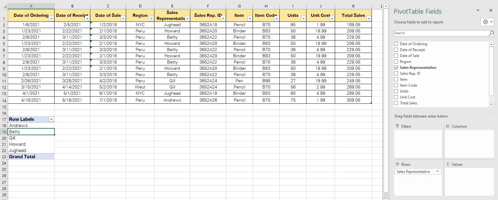
The image below represents a set of data that has multiple columns to it.

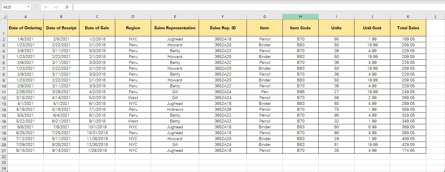
From the data above, you might want to see the results for Sales Representative ‘Jughead’ only.

Step 1:

How can you instantly filter out the data relevant to Jughead only?

To do so select the data and apply filters to your data as follows.

Select the data > Data Tab > Sort & Filter > Filters

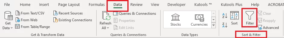
This applies filters to each column.

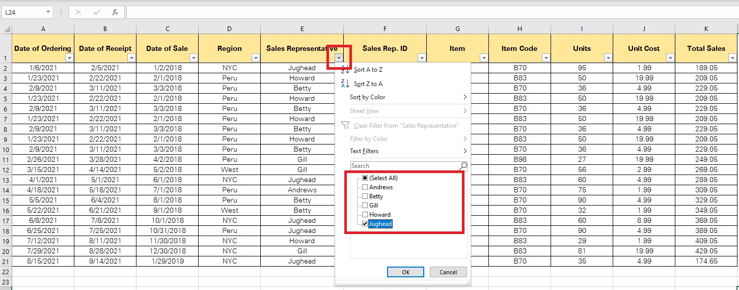
From the above data, you can click on each drop-down button and select the data type that you want to be filtered.

Step 2:

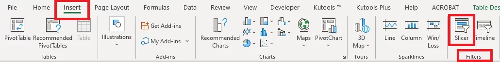
Now is the time to add slicers. To add slicers to this data, select the table or any cell from the table and go to:

Insert > Filters > Slicers

This opens up the ‘Insert Slicers’ dialogue box, as shown below.

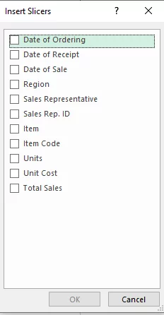
Step 3:

From the above pane, select the data column where you want to apply the filter.

In our example, we want to apply filters to the ‘Sales Representative’ column only, so let’s select that.

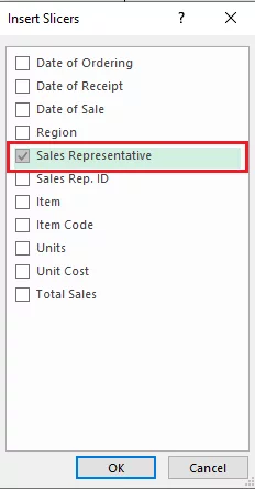
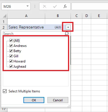
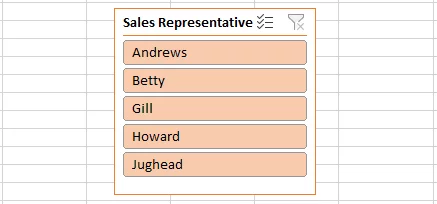
This adds a ‘Sales representative’ slicer to the data as shown below.

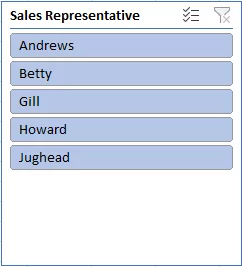
And that’s it. You can navigate between different sales representatives to see the data filtered out for each of them.

Pro Tip!

You can add multiple slicers to an Excel table and apply multiple filters together.

For example, you want to see sales records of Howard in NYC. This takes two data filters:

1. Sales Representative
2. Region

Inserting Multiple Slicers In A Pivot Table

The above section demonstrates how easy it is to insert slicers in an Excel table. Continuing the same, it’s time we see how slicers might be added to a Pivot Table.

Before we continue learning about inserting slicers into a Pivot Table, what is a Pivot Table?

An Excel Pivot Table is an advanced function in Excel used to summarize heaps of data into a single small table.

While Pivot Table eases out the job of Excel users greatly, adding slicers to it would do wonders for data analysts. This is particularly important if you need to make sense of the data within a single glance.

Adding multiple slicers to an Excel pivot table is super easy.

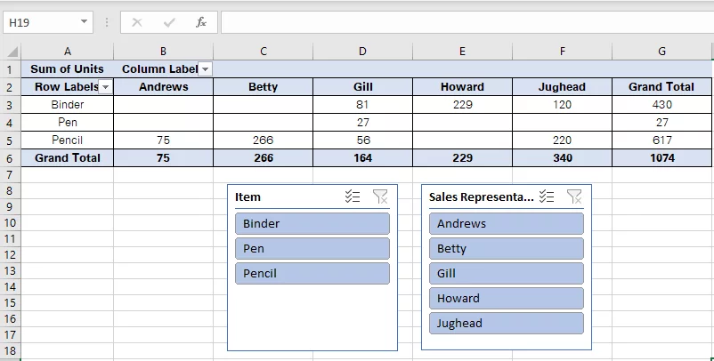
The image below represents a Pivot Table that summarizes the sales of different items made by different sales representatives.

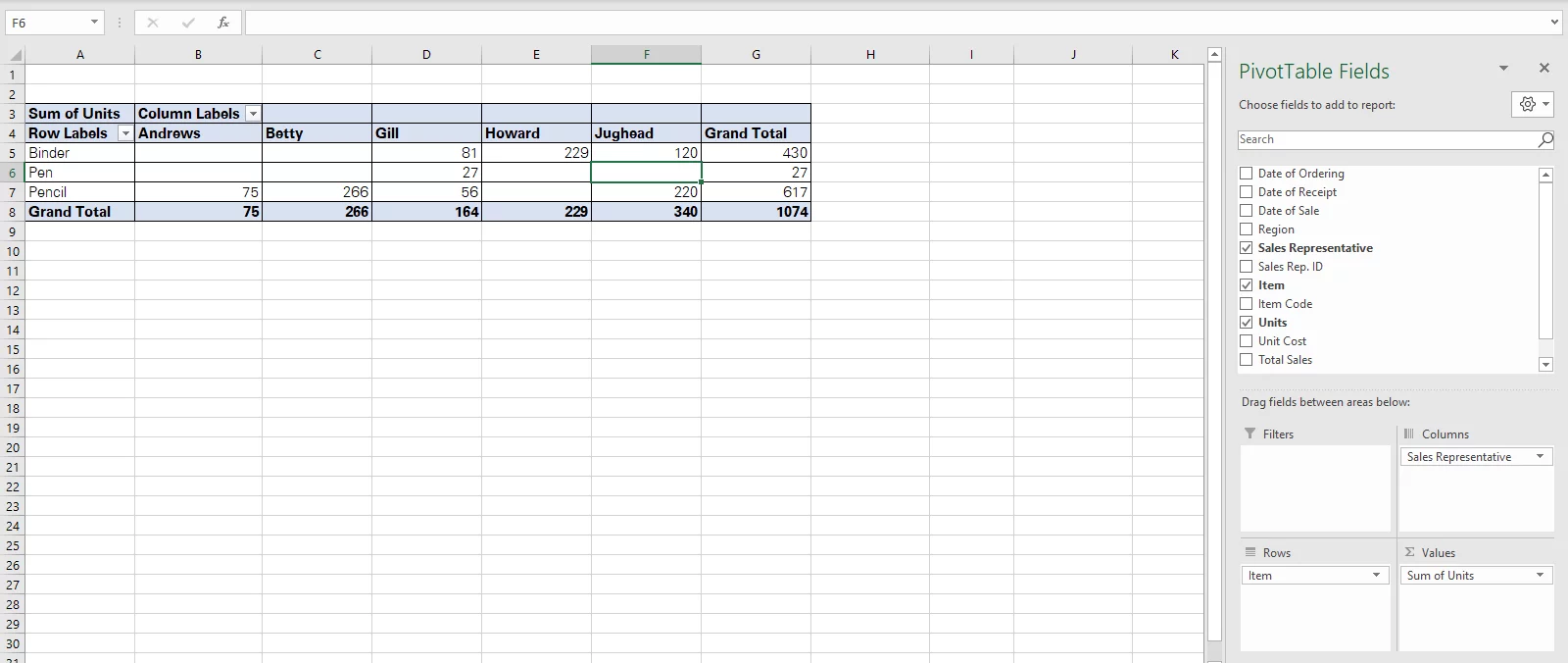
Sales representatives come row-wise, whereas the items sold by each of them are arranged column-wise.

To add slicers to this Pivot Table, follow the steps below:

Step 1:

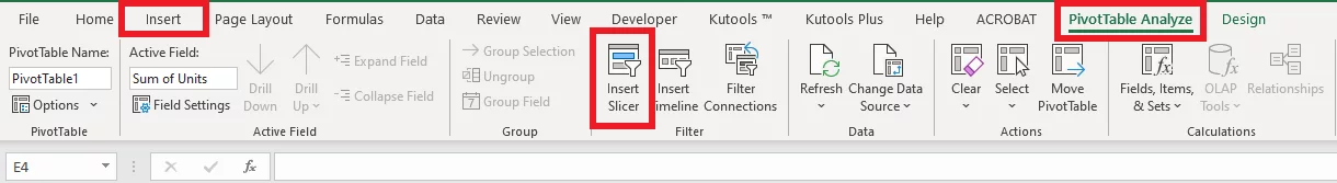
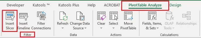
Click anywhere on the Pivot table and go to:

PivotTable Analyze > Filters > Insert Slicer

This opens up the Insert Slicers dialog box as follows:

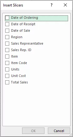
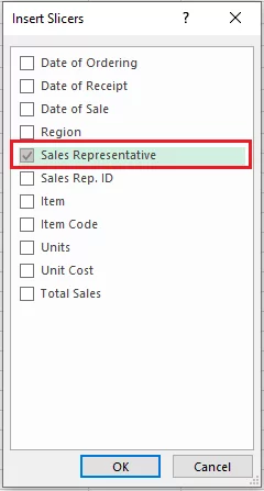
Step 2:

From the ‘Insert Slicers’ dialogue box, tick-mark the headers for which a slicer is to be added.

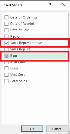
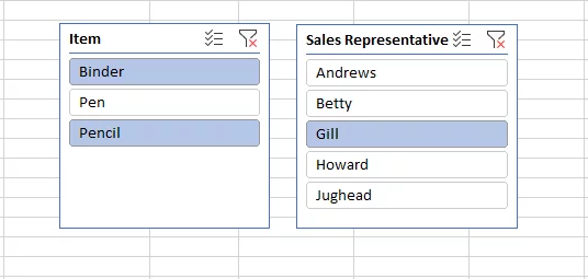
We have checked the checkbox for Sales Representatives and Item to add slicers for both as shown below.

Step 3:

And there you have your slicers added. From each slicer, choose from the several options to have the filtered results displayed.

For instance, to see the sales made by Gill, select Gill from the Sales Representatives slicer.

To further see only the sales of Binders made by Gill, select the said item from the Items Slicer.

Pro Tip!

To select multiple options from each slicer, for example, Pencil and Binder simultaneously, hit the control button while you select the second option.

How To Connect A Slicer To Multiple Pivot Tables / Pivot Charts?

It is often the case that your spreadsheet has multiple Pivot tables.

For example, take a look below.

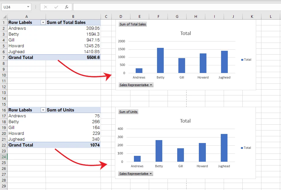
There are two pivot charts in the above image.

The first one (above) shows the total sales made by sales representatives. The second one (below) shows the units sold by sales representatives.

Step 1:

Click on the first Pivot Chart (for total sales) > PivotTable Analyze > Insert Slicers.

Add a slicer for Sales representatives.

Step 2:

Try filtering the data using the slicer.

This only brings changes to the first Pivot Chart. What if we want both the Pivot Charts to react to the same Slicer?

To make this happen, we need to connect both Pivot Charts to the Slicer.

Step 3:

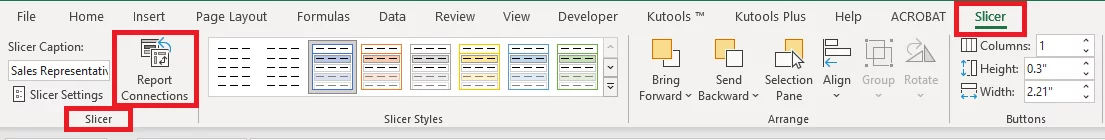
Click on the Slicer. Go to Slicer on the Ribbon > Slicer > Report Connections.

 

This opens up the connections box. Check the box for the second Pivot Table.

Step 4:

Now the same Slicer bears a connection to both the Pivot Tables (and the Pivot Charts). See below.

Doing so, if you make multiple pivot tables or pivot charts out of the same data, you can insert a single Slicer.

Formatting Slicers

Who said slicers are only about a blue-and-white set of options, and that’s it? You can always add different colours and formats to your slicer as needed.

Using the options in Excel, you can easily change the feel, style, look, and colours of Excel Slicers.

Why Would You Want To Format Slicers?

Slicers are used to apply quick filters to data. You might need to format slicers to glue them into your data.

For instance, below is a dashboard with a dark theme contrasting with orange. Adding a slicer with the default formatting (blue and white) might distort the look of the whole data.

However, after the slicer is formatted to the theme colours of the dashboard, the big picture looks much better.

There are many reasons you may want to edit the format of a slicer to your choice.

To learn how you may do it, let’s take the Slicers from the example above.

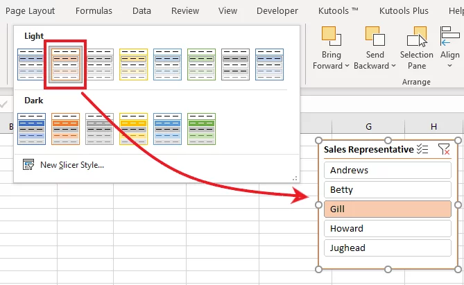
These Slicers are in the default slicer tone of Excel. To change the format of these slicers, click on any of these Slicers. This will add a new tab to the Ribbon by the name of Slicer.

Go to Slicer Styles and the thumbnail button on the right bottom.

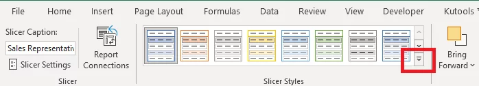
This opens up a drop-down menu of different Slicer Styles. Click any of them to have your Slice formatted accordingly.

If you want to go a step ahead, click on the option ‘New Slicer Style’ to see the dialogue box given below.

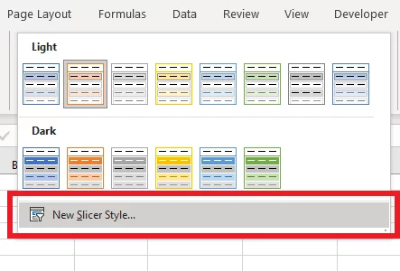
Browse through different options to customize the slicer as per your choice.

Adjusting The Height And Width Of Buttons

A slicer is like a table with some buttons on it.

These buttons make the look of the slicer, and you can customize their layout as desired.

To change the height/width of buttons:

Select the slicer > Go to Slicers > Buttons > Height / Width

Specify a height of your choice to have the slicer buttons adjusted accordingly.

For example, check out below.

Adjusting The Number Of Columns

Not only the height but you can also make changes to the number of columns of buttons per slicer.

To adjust the number of columns per slice:

Select the slicer > Go to Slicers > Buttons > Columns

This depends upon whether you want the slicer to be vertically styled or horizontally styled.

Adjusting The Height/Width Of The Slicer

After you’ve adjusted the height/width of the buttons within the slicer, you can also adjust the height of the slicer itself.

To adjust the height of the slicer

Select the slicer > Go to Slicers > Size > Height / Width

You may set the slicer to be in a vertical shape (more in height) or a horizontal shape (more in width).

After you’ve formatted all your slicers and everything else, how unfortunate would it be if you accidentally lost it all? This could be because you forgot to save your Excel file or were unable to recover an unsaved file. To learn all hacks to recover an unsaved Excel file, read out our article on recovering unsaved Excel files here.

Slicers Vs. The Report Filters

This section has a comparison between slicers and report filters. But before that let’s see what are report filters.

What Are Report Filters?

Report filter is an in-built function of Excel Pivot Tables. See below.

Using report filters you can focus on specific portions of your data by filtering out data.

To understand what report filters are and how they work, let’s consider the example of the Pivot Table below.

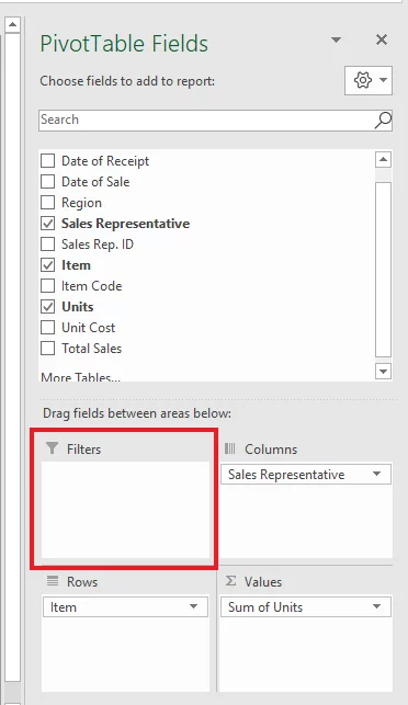
For instance, to apply report filters on sales representatives, drag and drop them to the Filter field, as shown below.

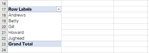
This changes the Pivot table to the following shape.

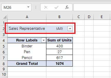
We see a drop-down menu with the name of the Sales Representative at the top.

But how does this help? Report filters can be used to filter out data for a particular sales representative only.

For example, we have the Items with their corresponding sales in the Pivot table.

From the sales representative drop-down menu, you may select any sales representative. Doing so, Excel would display results only for that one sales representative.

Hereabove, we selected Betty from the sales representative filter. Excel has filtered out the sales made by Betty.

The results show that Betty has only made sales of Pencils (266 units).

Report Filters Compared To Slicers

It’s time we compare report filters to slicers to see which one’s better.

To see this, let us see how slicers would have worked in the same situation above.

Step 1:

To add slicers to the above Pivot table, click anywhere on the Pivot table.

Go to PivotTable Analyze > Filter > Insert Slicer

Step 2:

This launches the ‘Insert Slicers’ pane. To apply filters to sales representatives, check the box for ‘sales representatives.’

This creates a slicer for ‘Sales Representatives’ as shown below.

How To Use Slicers With A Pivot Table?

You can also format the Slicer in different colours and themes to delve into your Excel sheet better.

Also, it is more interactive as you can readily choose different filters.

So Which One Is Better? Slicers Or Filters?

To know which one is better, let’s perform a quick comparison.

Report Filters	Slicers
Clumsy. Make the spreadsheet a little too complicated.	Visually appealing. Feel like interactive buttons on the screen.
Can only bear a connection to one Pivot Table.	Can be connected to multiple Pivot Tables at the same time.
Have a specific position within a column or row.	Can be moved around the spreadsheet like objects.
Takes a single cell.	Might take up too much space.
Can’t change the format.	Can be formatted to add different colours/themes in line with the spreadsheet.
Might prove chaotic to switch between filters during live presentations.	Are great for live presentations.

An additional way to filter data is by using the FILTER function – learn all about it here.

Using A Formula To Capture Slicer Selection

We have come across so much about slicers and their use in Excel. But can we use Slicer selections in formulas?

To understand what it means by using slicer selection in formulas, go through the example below.

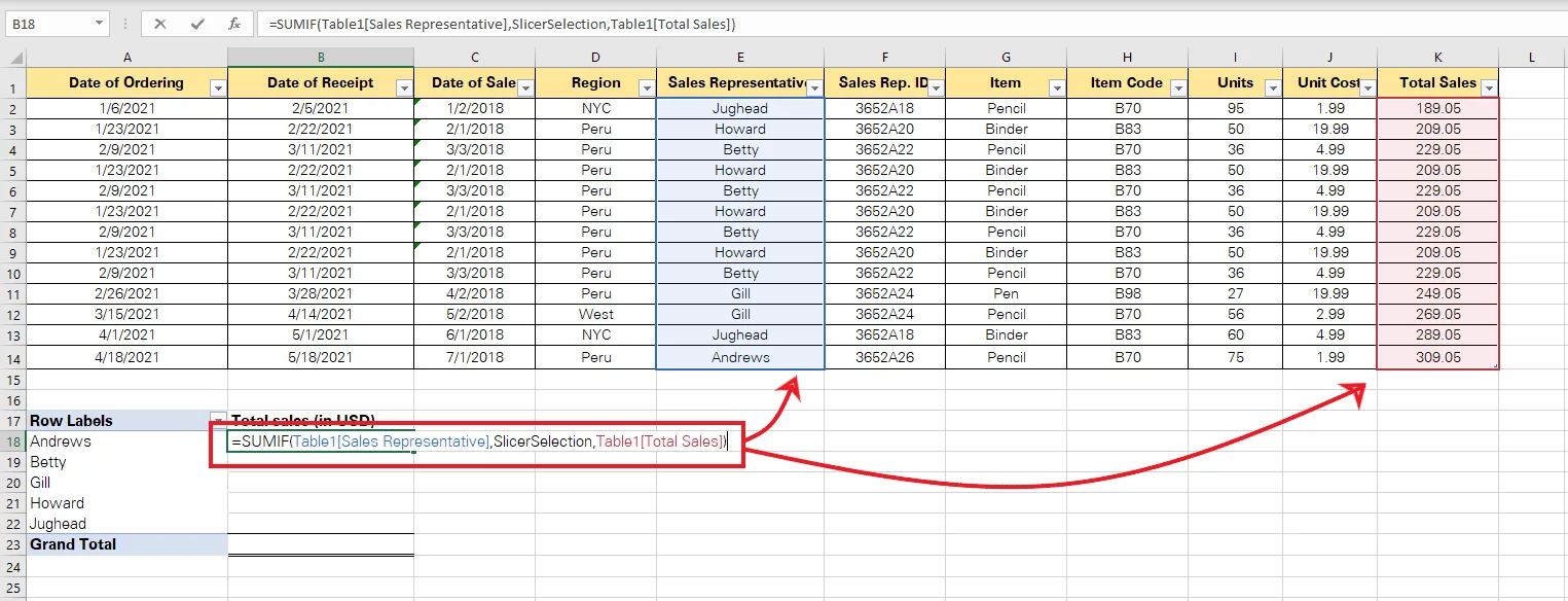
The image below represents the pivot table for different sales representatives.

For a quick reminder, this pivot table originates from source data (pivot table data) shown below. This data contains a column for total sales too. We want the sum of total sales made by each sales representative.

Now, let’s say we want to find the sales (in dollars) made by each sales representative below.

We can set up a formula for Excel to automatically identify it.

Step 1:

Name the range where the filtered sales representative appears. This will help us create a reference for it.

Select the cell where the name appears and name the said range ‘SlicerSelection’ or something else.

 

We have created a reference to ‘SlicerSelection’ as the criteria (second argument).

This is because we have named the cells (where the filtered results appear) as SlicerSelection.

Step 2:

Once done, let’s set up the SUMIF formula that uses the slicer selection.

Let’s write the SUMIF formula as follows.

= SUMIF (Table1[Sales Representative], SlicerSelection, Table1[Total Sales] 

What have we done?

• • The first argument of the SUMIF function specifies the range to be checked. In place of this argument, we have created a reference to the Sales Representatives in the source Table.
  • The second argument refers to the criteria to be looked for. We want the sum to be only performed for the filtered sales representative. This argument is set to SlicerSelection (the name we gave to the filtered results).
  • The third argument of the SUMIF function refers to the range to be summed up. As we want to see the total sales, we have created a reference to the Total sales column in the source Table.

Step 3:

All set. Press enter to make the formula work as follows.

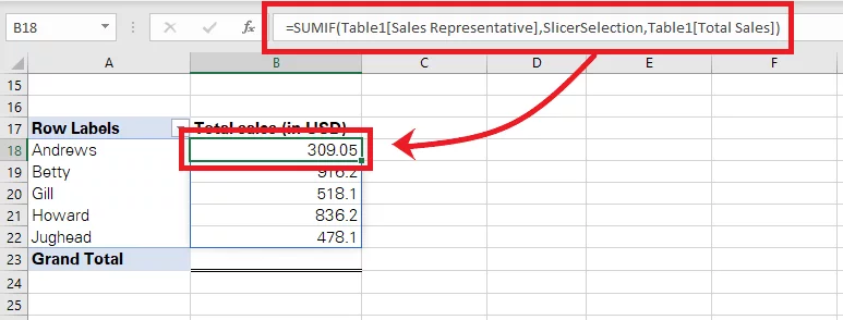
When we use the slicer to filter out any sales representative, the SUMIF function also filters out the result for only that sales representative.

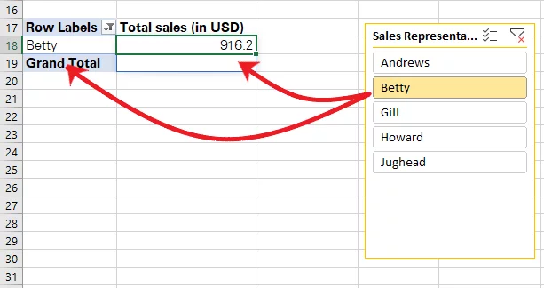
For example, select Betty from the above slicer, and the total sales would be accordingly filtered for Betty only.

This is how you can use Slicer selections in multiple formulas.

Pro Tip!

Must know that this is an Excel Array formula.

Troubleshooting:

Inserting and operating Slicers in Excel won’t cause you much trouble. However, some common problems are faced by users.

i. Changes To The Data

Slicers are only of use if they help the useful dissection of data.

You might make any changes to the source data, which may have a potential impact on your slicers. For example, in the example above you may include a new ‘Sales Representative’ to the source data.

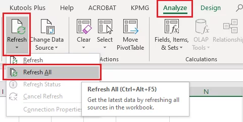
If the Slicers in your workbook do not immediately update to reflect the said change, go ahead and refresh the Pivot table.

To refresh the Pivot Table, click on any PivotTable, go to PivotTable Analyze > Data > Refresh > Refresh All.

ii. Slicer Moves With The Cells

A slicer is more like an object on the screen that will move as you drag it. Often when you reposition or resize the cells in the background, the slicer would also move. Or, if you delete the cells in the background, the slicer might also be lost.

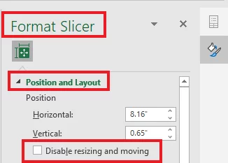
To save yourself from this problem, right-click on the Slicer.

Go to Size & Properties > Position & Layout

There are three options to fix the Slicer in place.

If you don’t want the slicer to move at all when the cells in the background are moved or repositioned, you may choose the option ‘Don’t move or size with the cells’.

iii.Lock The Slicer In Place

When making dashboards, you do want the slicers on the face of your dashboard. However, if you want to circulate the dashboard to others, you might prefer the Slicer to be locked in place.

This means users can operate the slicer but not move it or resize it.

This can particularly be helpful if you want the whole screen to be locked in place with the items no more being repositioned.

To lock the slicer in place:

Go to Size & Properties > Position & Layout

iv. Printing Slicers:

Slicers are of use in a spreadsheet where you can readily choose between different datasets to filter your data. However, when printing Excel reports, you might want to let go of the slicers.

Excluding slicers from printing is simple.

Go to Size & Properties > Properties

Uncheck the button for ‘Print object’ and you’re all good to go!

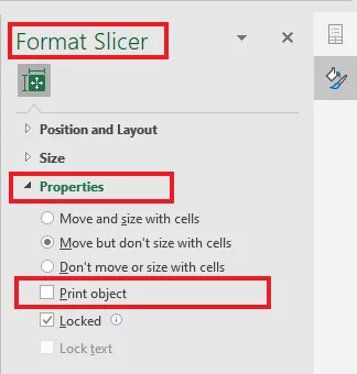
Hit ‘Ctrl + P’ for a quick check to see if the slicer appears in the print view.

 

Conclusion

If you’ve ever used Pivot Table / Pivot Charts in Excel, you’d know how useful slicers can be. Not only for Pivot Tables, but you can also use the same for Excel tables.

Slicers make spreadsheets more interactive, and easier to use. You can readily apply filters to data and switch between them.

Also, as a Slicer can be connected to multiple Pivot tables, it becomes all the more useful. The above article is all about Slicers in Excel.

Keep practising using the examples above and more to become a pro in Excel.