Ultimate Guide to Advanced Filters in Excel

 

Excel Advanced Filters are one of the main reasons why people prefer using Microsoft Excel for most of their work – be it data recording, analysis, or presentation.

But to your surprise, the simple filter of Excel is not even close to Excel Advanced Filters in terms of advancement of features.

What’s even more surprising is the under-usage of this stunning tool.

The main reason for Excel Advanced filters being underrated and underused is their less familiarity among the Excel audience.

Continue reading through this guide to know all about Advanced Filters in Excel.

What Are Advanced Filters?

Advanced filters help you sort your data, which we recommend you do before creating graphs from it.

However, advanced filters offer a wide variety of advanced filtering options in addition to common filtering.

Some of these are as follows.

• Advanced filters allow you to extract unique data sets of your choice and export them to different locations other than the original file.
• You can define complex logical criteria. Excel would identify and filter out data based on the defined criteria.
• It also allows users to define multiple ‘AND’ and ‘OR’ criteria for filtering out records that fit their needs.

Using Advanced Filter to Extract a Unique List

You can use the Advanced Filter function to extract a unique list of values out of a given dataset.

Let’s take a look at the example below to find out how.

Below is a screenshot that manifests a dataset containing multiple duplicate values. The same has been highlighted for your ease of reference.

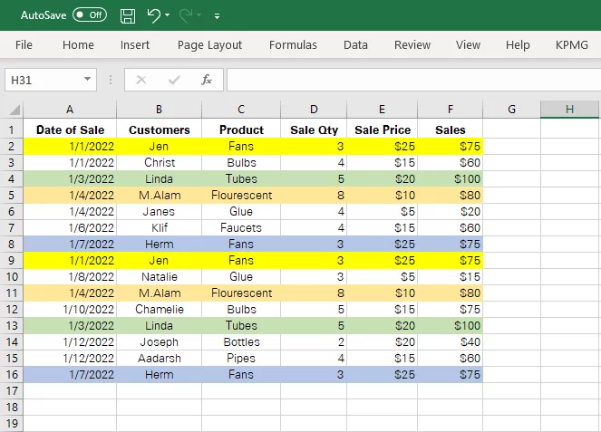
The advanced filter of Excel is great for filtering data, but it can also help you remove duplicate values.

To filter only a unique set of sales records from the dataset given above, here are the steps to be followed.

Step 1:

Select the data to be filtered and open the Advanced Filter Dialogue Box as follows.

Data > Sort & Filter > Advanced

This would open up a dialogue box as follows.

 

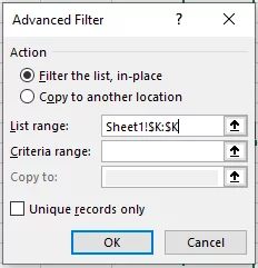
Pro Tip: Alternatively, you can use the shortcut key [Alt + A + Q] to reach out for the Advanced Filters dialogue box.

Step 2:

From the Advanced Filters Dialogue box, make the following choices.

• • Action:

If you want your original dataset to be filtered of unique values, select the option ‘Filter the list, in place’.

On the contrary, if you want the original dataset to remain unchanged and only a unique copy of the dataset to be extracted, select ‘Copy to another location’.

• • List Range:

List range refers to the original data set from where a unique list is to be extracted. Make sure to include headers in it too.

• • Criteria Range:

As we are not specifying any criteria in this example, the criteria range is to be left empty.

• • Copy to:

Until and unless you check the ‘Copy to another location’ option appearing under the Action tab of the dialogue box, this box would be frozen.

This is because it refers to the destination location where you want the data to be exported in case you want to extract it to a different location.

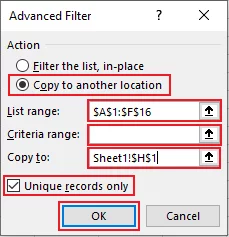
In the current example, we have selected the cells containing the data under the listed range. Under Action, we have selected ‘Copy to another location’. Accordingly, the destination address is populated in ‘Copy to’.

What filters out the duplicate values is the option at the bottom i.e. Unique records only. When checked, Excel copies the same data to the destination address except for the duplicate values.

The results are as follows.

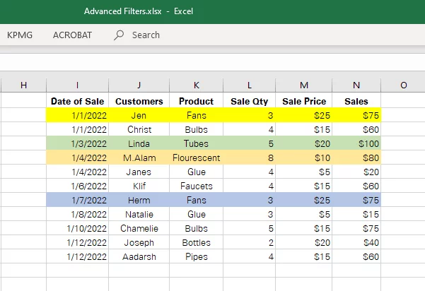
Note: Using ordinary duplicate value removal techniques helps you remove duplicates and makes the edits directly to the original data. However, through advanced filters, you can extract a unique record to a new location without making changes to the source file.

Advanced Filter Use Cases

Despite being one of the most underused features of Excel, advanced filters can come in handy for several purposes. Go through a few use cases below to see how you may employ advanced filters to help your Excel jobs.

• Often businesses have a specific code allocated to each employee. This might consist of a special alphabet or number. For example, all employees of the sales department might have the code SAL like SAL2544.

To filter out employees of the sales department from the list of all employees, you may define the criteria using a wildcard character as ‘SAL*’. Doing so, Excel would filter out all employees having the code ‘SAL’ in their employee code.

• To keep track of perishable items that are close to their expiry date, bakery businesses keep a record of manufacturing dates of all eatables.

Defining an ‘AND criteria’ by mentioning ‘Bread’ under the header Product and a 10 days old date under the header Manufacturing date, the number of items near expiry can be easily tracked.

The advanced filter can be used also be used to find outliers in a large dataset.

Once you know the underlying science, you’d know how easy yet useful this function can prove to be.

Criteria And Logical Operators

Ready to come across some cool features of Excel? Here you go. There’s just so much you can do using Advanced Filters in Excel.

Using criteria and logical operators in advanced filters, you can filter data in different ways. To brainstorm a little, we have compiled below a list of some common comparison operators that you can use to define a criterion.

Operator	Meaning
=	Equal Sign
>	Greater than
<	Less than
>=	Greater than or equal to
<=	Lesser than or equal to
<>	Not equal to

 

To see how you may apply these logical operators to constitute a criterion, follow the example below.

The AND Criteria

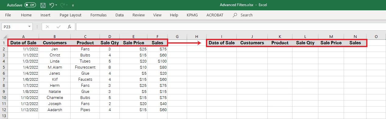
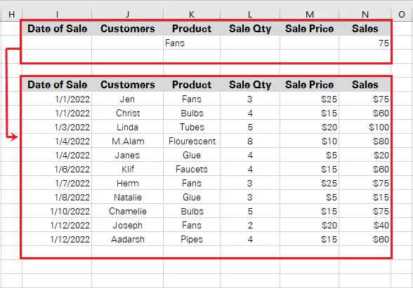
The screenshot below shows sales made to different customers along with other ancillary details.

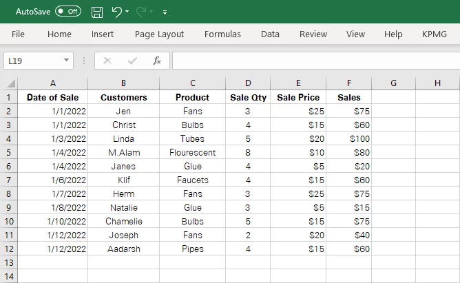
Out of this record, you may only want to extract transactions of sales of fans where the Sale quantity is 3 or more. Filtering such results requires us to define two criteria that are to apply to the data simultaneously.

Defining more than one criterion where Excel returns results only when all the criteria are ‘TRUE’ is called AND criteria. In simpler words, we tell Excel to return results with transactions that meet both the first and the second criterion.

To do so, follow the simple steps below.

Step 1:

Copy and paste the headers of your data to a separate location (in the same sheet). These headers would then be used to specify the criteria.

Step 2:

Under each header, specify the criteria based upon which you want the data filtered. In our stipulated example, we have two criteria.

1. 1. 1. Under the header ‘Product’, we want ‘Fans’ to filter out sales of fans.
      2. Under the header ‘Sale Qty’, we want sales that are equal to or greater than 3. In terms of logical operators, ‘>=3’.

Specify the criteria under each respective header as follows.

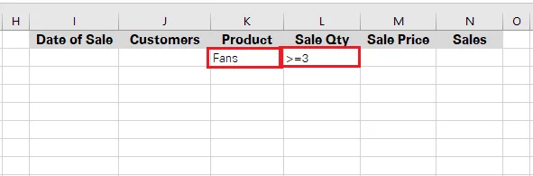
This now serves as the criteria for your advanced filter search.

Step 3:

Select the source dataset (with the headers) and reach out for advanced filters through Data > Sort & Filter > Advanced.

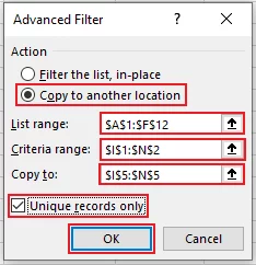
Once the advanced filters’ dialogue box opens up, choose the options as follows.

1. 1. 1. Copy to another location – Select this option.
      2. List Range – This must include the cell range containing the original dataset along with the relevant headers.
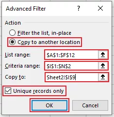
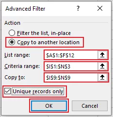
      3. Criteria Range – This includes the cell where the advanced filter criteria are specified. In our example the criteria range is I1:N2.
      4. Copy to – Specify the location where you want the filtered results to appear.
      5. Unique records only – check this option.

Here is what the advanced filters’ dialogue box should look like once all populated.

Hit ‘OK’ to have filtered data as follows.

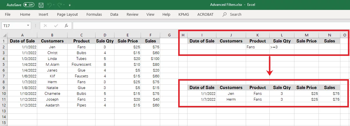
Excel has filtered out those entries where sales of ‘Fans’ were booked and sale quantity was equal to or more than three.

Advanced Filter Excel helps you perform a better analysis of data.

The OR criteria

After we practically demonstrated the application of AND criteria, let’s look into how ‘OR’ criteria works with Advanced filters in Excel.

Continuing the same example as above. You may want to filter out sales of Fans or Bulbs where the Sales amount to $75 or $40.

As both the conditions have an OR, this means excel must filter results if either of the criteria is met. To do so follows the steps below.

Step 1:

Just as above, copy and paste the headers of your data to a separate location (in the same sheet).

Step 2:

Under each header, specify the criteria based upon which you want the data filtered. In our stipulated example, we have two criteria to be specified.

1. 1. Under the header ‘Product’, add Fans in one row and Bulbs in the next row.
   2. Under the header ‘Sales’, add ‘=75’ in one row and ‘=40’ in the next row as we want sales to be equivalent to either 75 or 40.

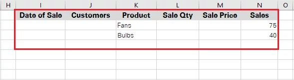
This now serves as the criteria for your advanced filter search.

Pro Tip: In Excel, any entry in a cell preceded by an ‘equals to (=)’ sign is interpreted as a formula. Excel then automatically applies the formula and displays the results in the cell. This is why in the screenshot above, there appears no ‘equals to’ sign before 40 or 75.

Step 3:

Select the source dataset (with the headers) and reach out for advanced filters through Data Tab > Sort & Filter > Advanced.

Once the advanced filters’ dialogue box opens up, choose the options as follows.

1. 1. Copy to another location – Select this option.
   2. List Range –Select the cells where the original date is located.
   3. Criteria Range Box – Select the advanced filter criteria range as I1:N3.
   4. Copy to – Specify the location where you want the filtered results to appear.
   5. Unique records only – check this option.

Here is what the advanced filters dialogue box should look like once all populated.

Hit ‘OK’ to have results as follows.

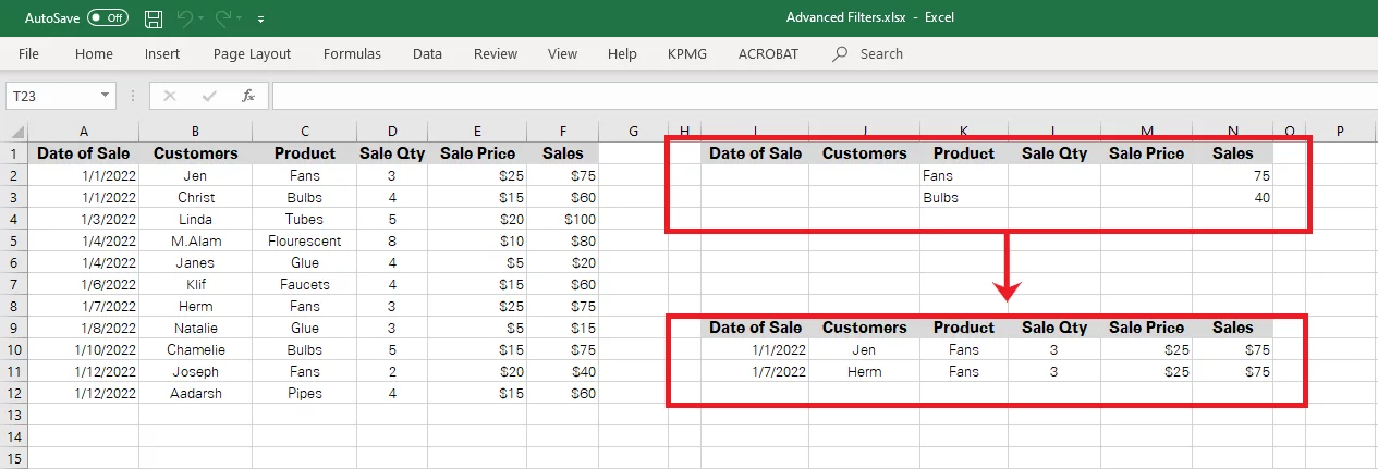
Excel has filtered out those entries where sales of ‘Fans’ or ‘Bulbs’ were booked, and sale quantity was ‘$75’ or ‘$40’.

Note: This example uses the logical functions ‘AND’ and ‘OR’, which can be used in all sorts of functions.

WILDCARD Characters

Wildcard characters are an advanced technique, covered on our advanced Excel courses.

There are three wildcard characters.

• Asterisk (*) – An asterisk stands for any number of characters starting from the position of the asterisk in a word. For example, ‘Fa*’ could denote ‘Fan’, ‘Fans’, ‘Fandom’ etc.
• Question Mark (?) – A question mark stands for any single character positioned against the question mark. For example, ‘F?n’ could denote ‘Fan’, ‘Fin’, ‘Fun’ but not ‘Fans’.
• Tilde (~) – A tilde is generally used for any wildcard character in a text.

How you may use them with Advanced Filters in Excel? Let’s see the example below.

From the same dataset as above, if you want to filter out sales made to all those customers whose name starts with ‘J’, you may define the criteria as follows.

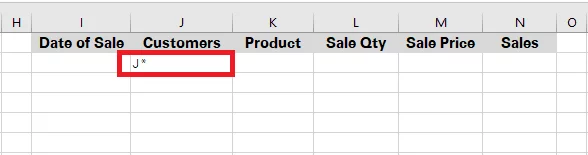
Step 1:

Under the header ‘Customers’, define the criterion as ‘J*’.

Step 2:

Next, apply advanced filters as follows.

Hit ‘OK’ to see results as follows.

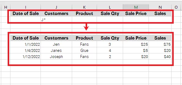
You may also use other wildcard characters to filter out required data and yield sophisticated results.

Troubleshooting for Advanced Filter

Advanced Filter of Excel is undoubtedly an easy-peasy function with so many uses. However, this doesn’t rid it of common troubleshooting problems. Some of the most commonly complained problems include the following.

1.   Not copying the exact headers

If your advanced filter is not working as intended, there is a high chance you wrongly copied the headers. As headers are used as criteria, they need to be the same as the headers in the original data set.

It is advised to copy/paste the headers from the original set. However, even if otherwise, you intend to manually make them up again, pay special attention to the spelling, as inconsistent spellings of headers can also render your filtration exercise invalid.

2.   Inappropriately defining the criteria

Another common error that users are often subject to is defining the criteria range inappropriately. For instance, for the example above, we have defined the criteria as follows.

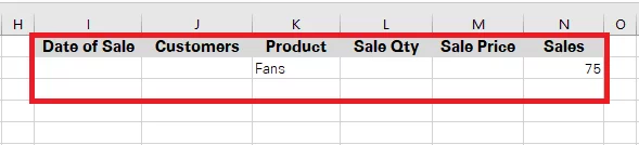
As is evident from the screenshot, the criteria fit a single row after the header. However, while defining the criteria, if you define the range as ‘I1:N3’, Excel would display these results.

This is because the range defined includes a redundant row and Excel also takes it as an OR criteria. To yield accurate results, make sure to define the criteria range precisely. For the example above, the correct criteria range for the above case is I1:N2 and not I1:N3.

Conclusion:

Data filtration is one of the most common needs of all regular and proficient Excel users. However, it can often get super laborious if you are not adept with the right technique to get the desired results.

Advanced filters of Excel can help you have your data aligned in numerous ways. Put together some data and try for yourself.