Create And Personalise Your Excel Dashboard!

In this tutorial, we will take you through the steps needed to create an Excel Dashboard. We will also review some best practices when it comes to dashboard creation and visualization.

An Excel Dashboard is a powerful visualization tool that incorporates charts and other interactive visual features, to display important business related insights.

If you would like to learn more about other advanced Excel features, then please consider joining one of our top-rated Excel courses.

 

Excel Dashboards Explained

You can create a dashboard using other popular data analysis software, such as Power BI, Tableau or Qlik. When you create a dashboard in Excel, you will leverage certain key features.

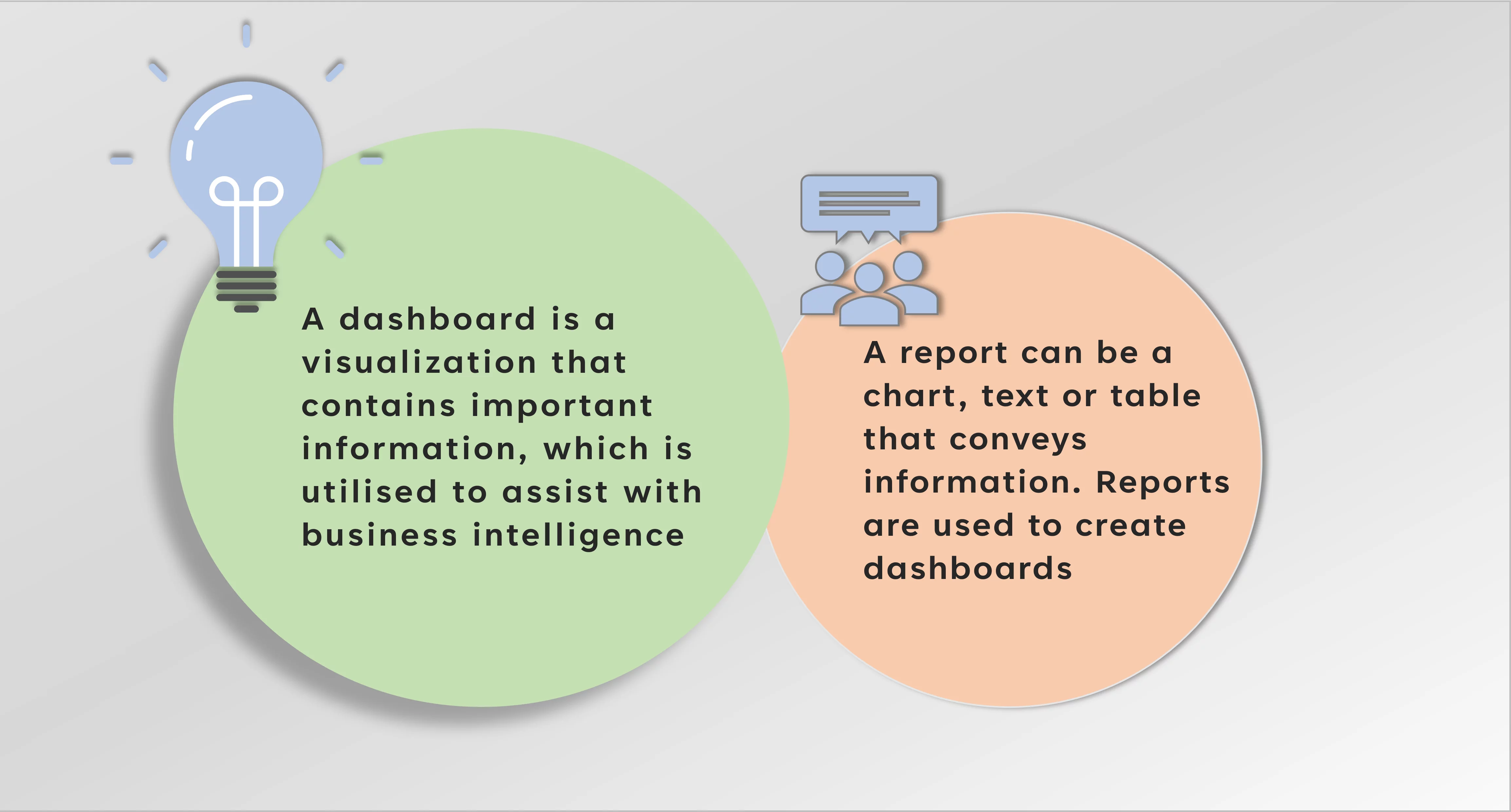
A dashboard should provide insights and assist the organization with making business decisions.

Using just PivotCharts, Slicers and graphics, you can create quite a sophisticated Excel dashboard. Alternatively, you can incorporate VBA for advanced functionality. In this tutorial, we will focus on the technique that utilises PivotCharts, a Slicer and graphics.

You may have heard the terms dashboard and report used interchangeably, so let’s review what the difference is.

 

If you would like to learn about how to create a dashboard in Power BI, then please read this post!

 

Planning Your Excel Dashboard

The first stage involved in Dashboard creation, is the Planning stage. Follow these easy steps for planning!

 

1. Consider the purpose of your prospective dashboard. The purpose will guide you, as you are creating the actual Dashboard. Since you maybe wondering about what information to include.

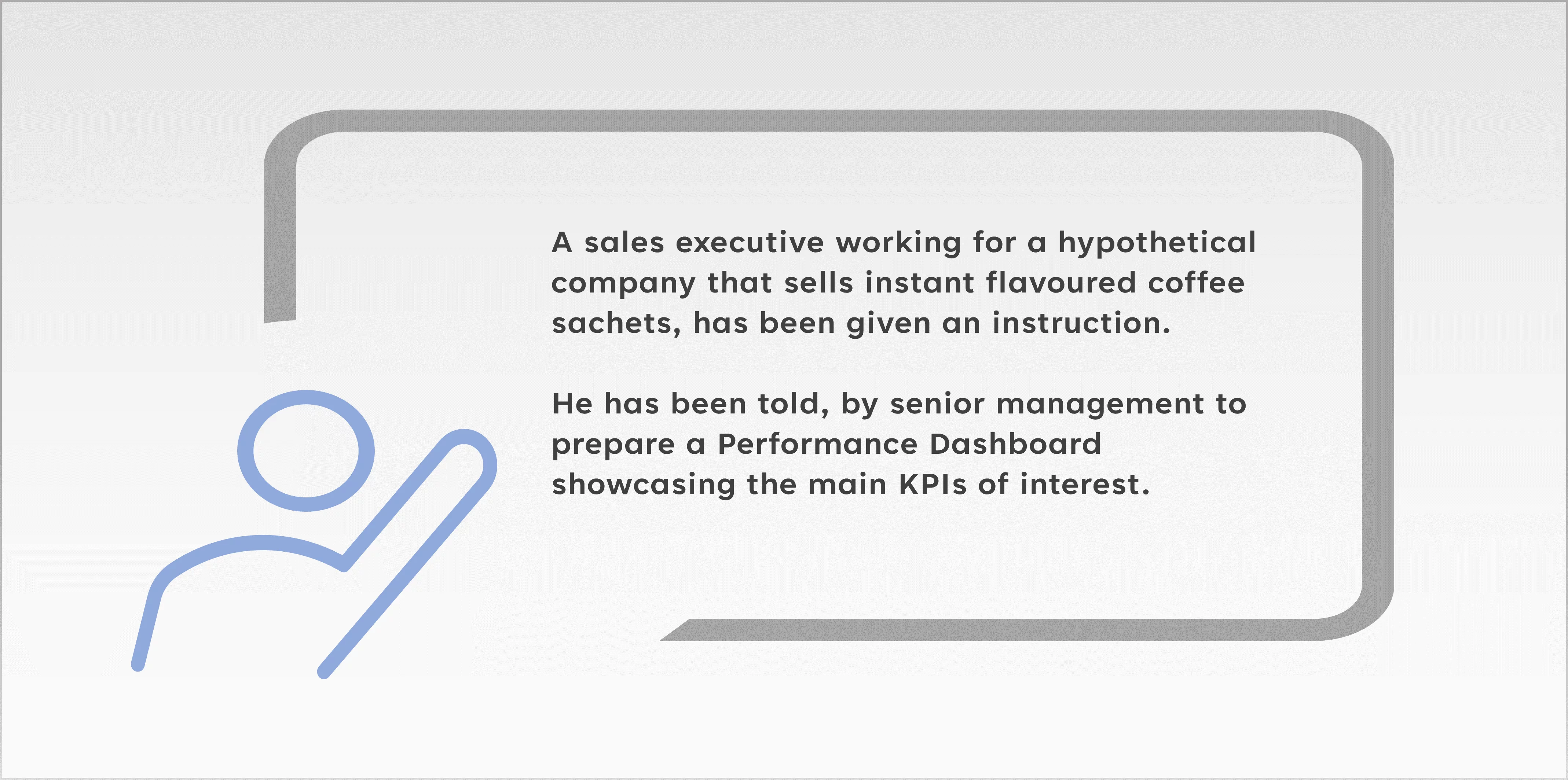
For example, let’s say a sales executive is given an instruction to prepare a Sales Dashboard. So, the purpose of the dashboard is to showcase the main sales KPIs and performance metrics. He may want to add a chart to his dashboard that shows the annual profits gleaned from each market. He may also want to include a graphic that highlights the top-selling products or top customers.

 

2.  You should also consider your audience and their skill level in Excel. For example, a financial analyst working with stocks could use an Open-High-Low-Close chart to display stock information. A biostatistician could use a histogram to display the frequency of certain eye colours, within a group from a specific area.

Ideally, one of your goals should be to create a user-friendly dashboard that conveys the key information, without the user needing to tweak the dashboard in any way

 

3.  It’s advisable to design an outline of your dashboard. You could use standard software such as PowerPoint or Word in order to create this outline. This will be a rough diagram of where you’d like to place your main visualizations (PivotCharts, Slicers and graphics).

 

4.  Think about the colour scheme,  font combination and any other graphics that would be appropriate for your dashboard.

A good rule of thumb, when it comes to colour schemes is to keep it simple. Don’t use too many colours. You want your colours to emphasize your key points, not distract from them.

If you are designing a dashboard for your company, you may need to use your company’s colours.

Try not to use more than two fonts on your dashboard.

In terms of other graphics that are not charts, use these sparingly. Since you don’t want your dashboard to be too cluttered. If you are designing a dashboard for a company that sells tractors for example, you could include a very small graphic of a tractor next to the heading.

Tip: Review some dashboard templates and online tutorials to get ideas and inspiration for your dashboard.

 

The Tools and Resources You Need To Make Your Dashboard

You will of course need Excel to create your dashboard. Additionally, you can use sites such as unsplash.com or pixabay.com in order to find sheet background images.

For other graphical elements/images you can also use those sites. Office 365 users can make use of the Stock Images… option.

For colour palettes/schemes, you can look at sites such as coloors.co and view the Trending Color Palettes – Coolors page. You don’t have to use the entire palette. In fact it’s advisable to just pick a few colours from your palette of choice.

Alternatively, you can use the built-in colour palette in Office that comes with each theme.

 

Designing Your Excel Dashboard

The second stage involved in Dashboard creation, is the Design stage.

 

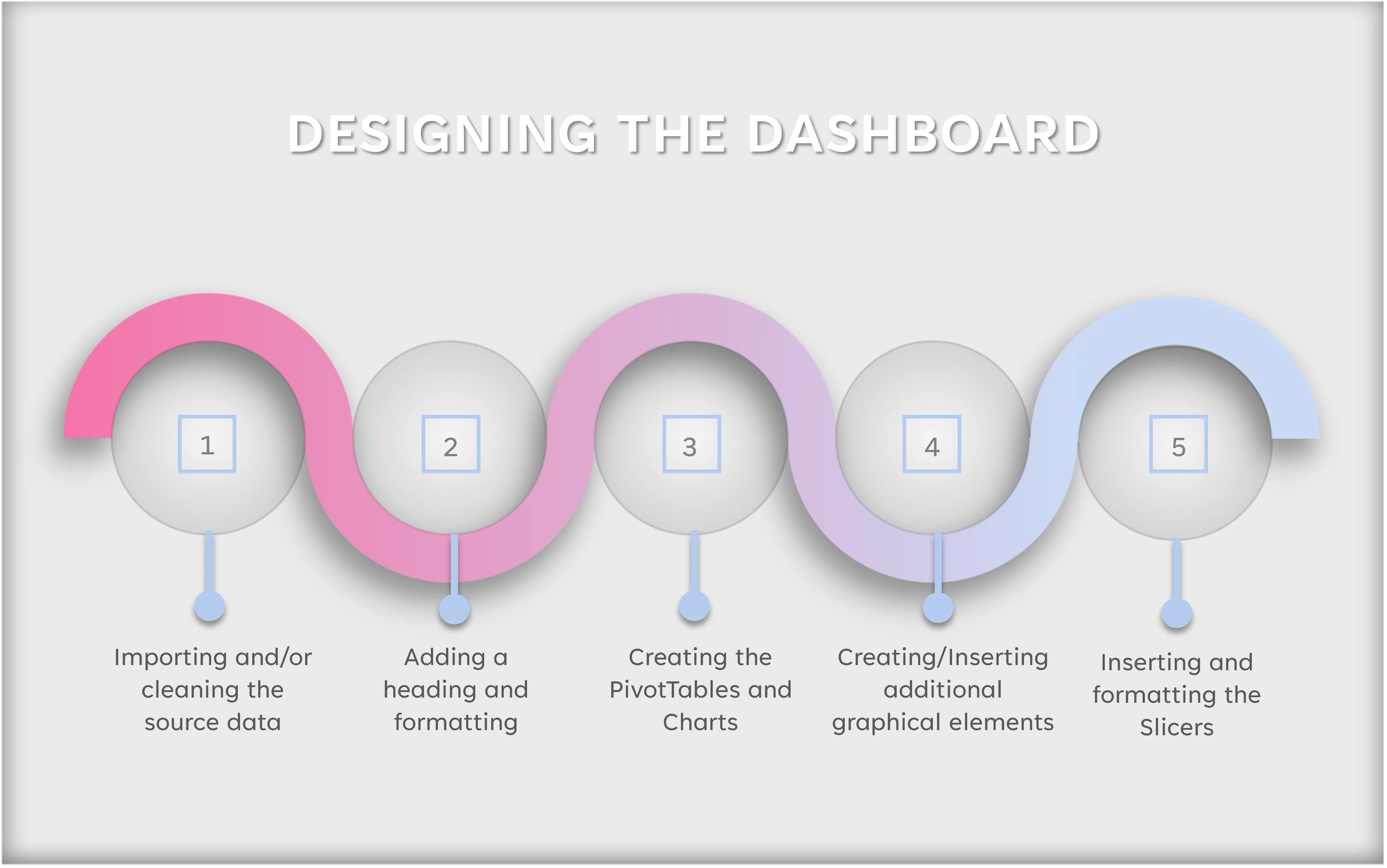
• • • Importing and/or Cleaning The Source Data

If your source data is already in Excel and cleaned, then you are set for the next step. If you are unsure about what data cleanup entails, then please visit this post on Removing Blank Cells.

Alternatively, your data may be stored in an external source such as a SQL Server database, in which case you will need to import your data. You can use Power Query to import and clean your data if necessary.

To learn more about how to use Excel Power Query, to automate the process of importing and cleaning data, read here!

 

• • • Adding a Heading and Formatting

It’s advisable to add a heading to your Dashboard sheet. Keep the heading short but descriptive, it should convey what the dashboard will be about. You should also add some basic formatting to your heading and a background colour to the heading section, if needed.

 

• • • Creating the Table, PivotTables and Charts

In most cases you need to have a primary data table. You will then create PivotTables from that primary data table. PivotCharts will be the main graphical visualizations of your dashboard, when using this technique.

You need to customize the PivotCharts according to your chosen colour scheme and font choice.

You will eventually add the PivotCharts to your Dashboard sheet and position them according to their placement on the outline.

 

If you would like to learn more about PivotTable creation, then please read our guide here.

 

• • • Creating/Inserting Additional Graphics

This is an optional step and involves creating/inserting any additional graphical elements other than PivotCharts and Slicers to the dashboard.

 

• • • Inserting the Slicers.

Slicers provide a way of adding interactivity to your dashboard. When the user clicks on a button on the Slicer, certain PivotCharts in the dashboard will be filtered accordingly. You will place the Slicer(s) in the position where it’s shown on the outline.

You can customize the Slicer(s) according to your needs.

 

Step-by-Step Dashboard Example

Let’s see how this works, by looking at a simple example. This is for a hypothetical start-up company that has been operating for six months.

 

 

The Planning Stage

• • • So, the purpose of the dashboard is to showcase the main metrics such as the most profitable flavours, the least profitable flavours and who the best customers are. He would also like to showcase the overall sales trend for all of the flavours.

 

• • • The audience and main users of the dashboard are senior management, who are interested in the performance of the different flavours of coffee sachets. They would like to use the Dashboard to assist with Business Intelligence. The Dashboard should be well designed and easy to use.

 

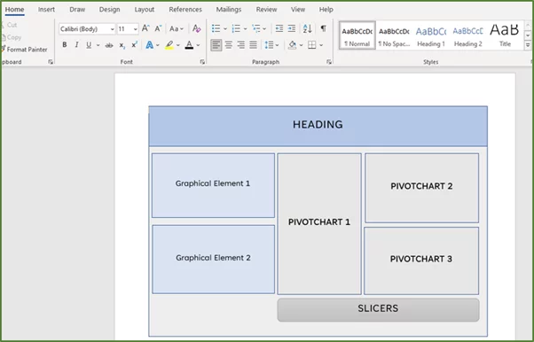
• • • The next step in the planning process is to design a simple outline of the Dashboard, in either PowerPoint or Word. In this case, we used Word. This is just a rough diagram that we are going to use to guide us, when designing the Dashboard. We created it using standard shapes and textboxes.

 

• • • For the colour scheme, we decided to go with some neutral greys and blues from the palette of the Office theme, for the most part. We will also use two other grey tones.

 

We have planned the Dashboard accordingly, so let’s look at the Design stage.

 

The Design Stage

Step 1

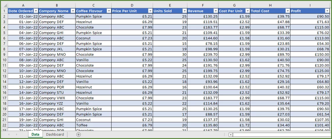
Let’s review our source data set. It’s already in an Excel workbook and has been cleaned.

 

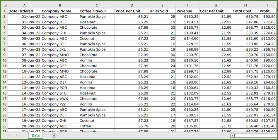
We have the sales data for our hypothetical company. It includes the following columns:

 

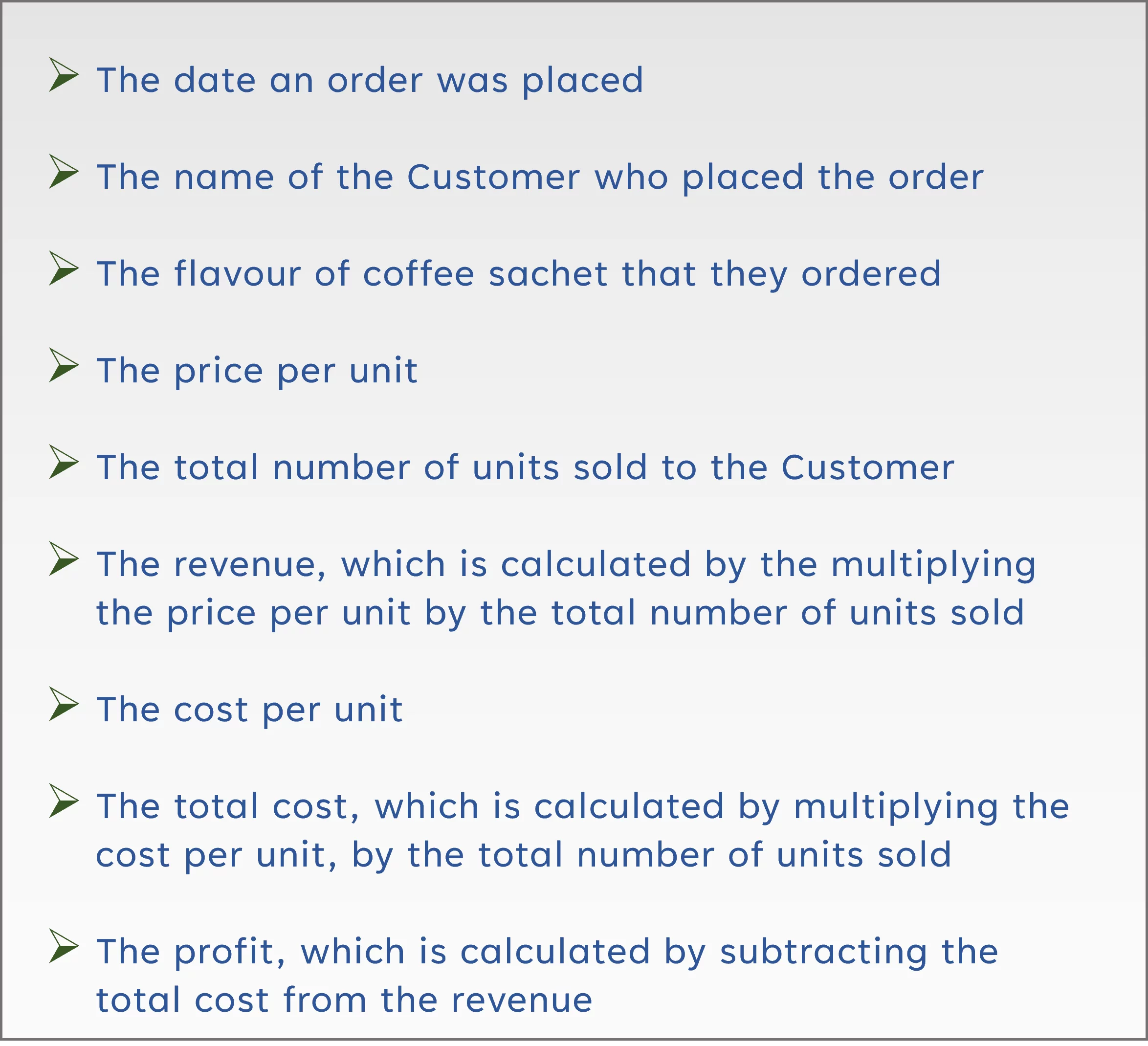
We have 193 rows of data including the headings. There are eight different flavours of coffee sachet. The data set is stored on a sheet called Data.

Step 2

We will create a new sheet and name the sheet Dashboard.

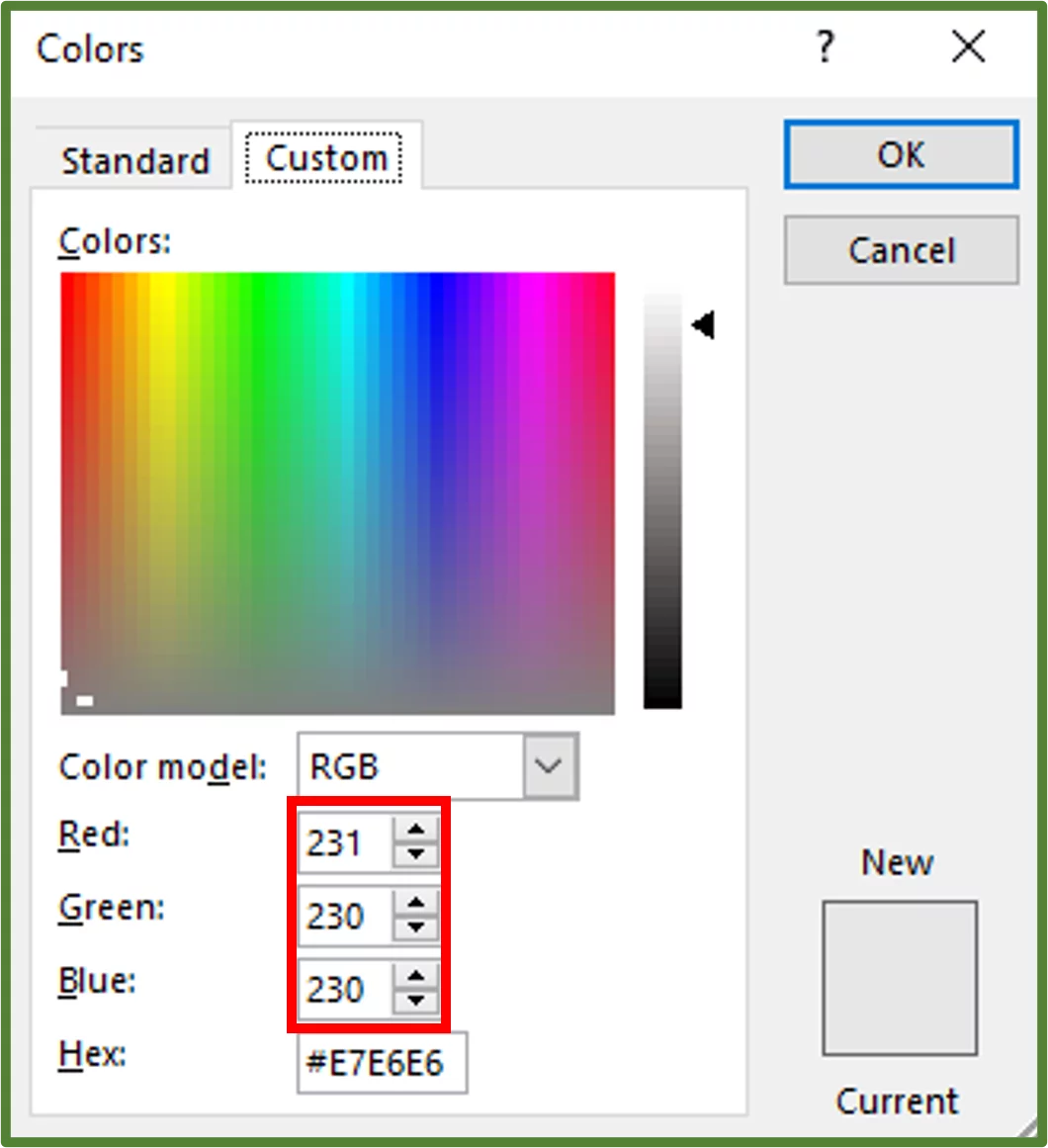
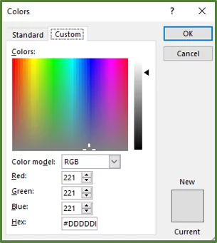
Select range A1:U2 and go to the Home Tab. In the Font Group, select Fill Color. Choose More Colours…

We would like a neutral grey colour. Using the Colors Dialog Box, select Custom and change the red value to 231, the green value to 230 and the blue value to 230.

 

Go to the Insert Tab, and in the Text Group, select TextBox.

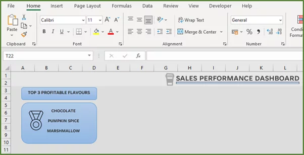
Draw a Text box on the Dashboard worksheet, over the grey background area. Type the words Sales Performance Dashboard in the Text box. Centre the Text.

With the Text box still selected, go to the Home Tab. In the Font Group, change the font to Tenorite. Increase the size to 16 and the font weight to bold. Change the font colour to Black, Text 1, Lighter 25%.

 

Tenorite is a new font available to Office 365 subscribers. For older versions of Office, you can use any Sans Serif font such as Calibri.

Select the  Text Box and go to the Shape Format Tab. In the Shape Styles Group, select Shape Fill and then choose No Fill.

Then select Shape Outline and choose No Outline.

Reposition the Text Box.

 

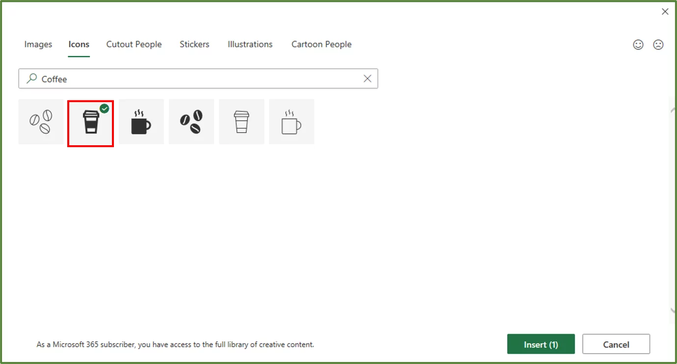
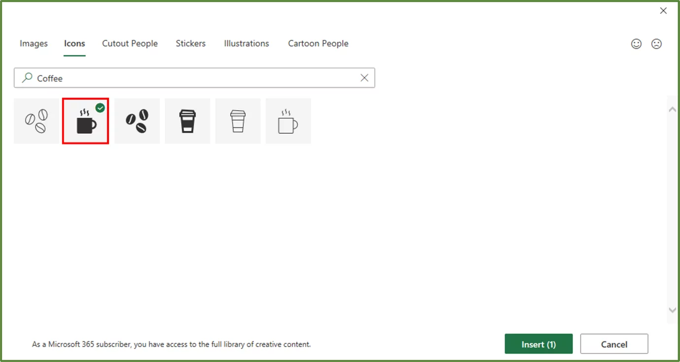
Now go to the Insert Tab and in the Illustrations Group, select Pictures. Choose the Stock Images… option.

 

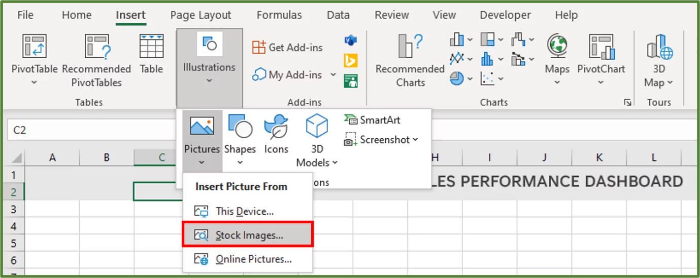
Select the Icons option and type Coffee in the Search Box. Choose the following image and click on the Insert Button.

 

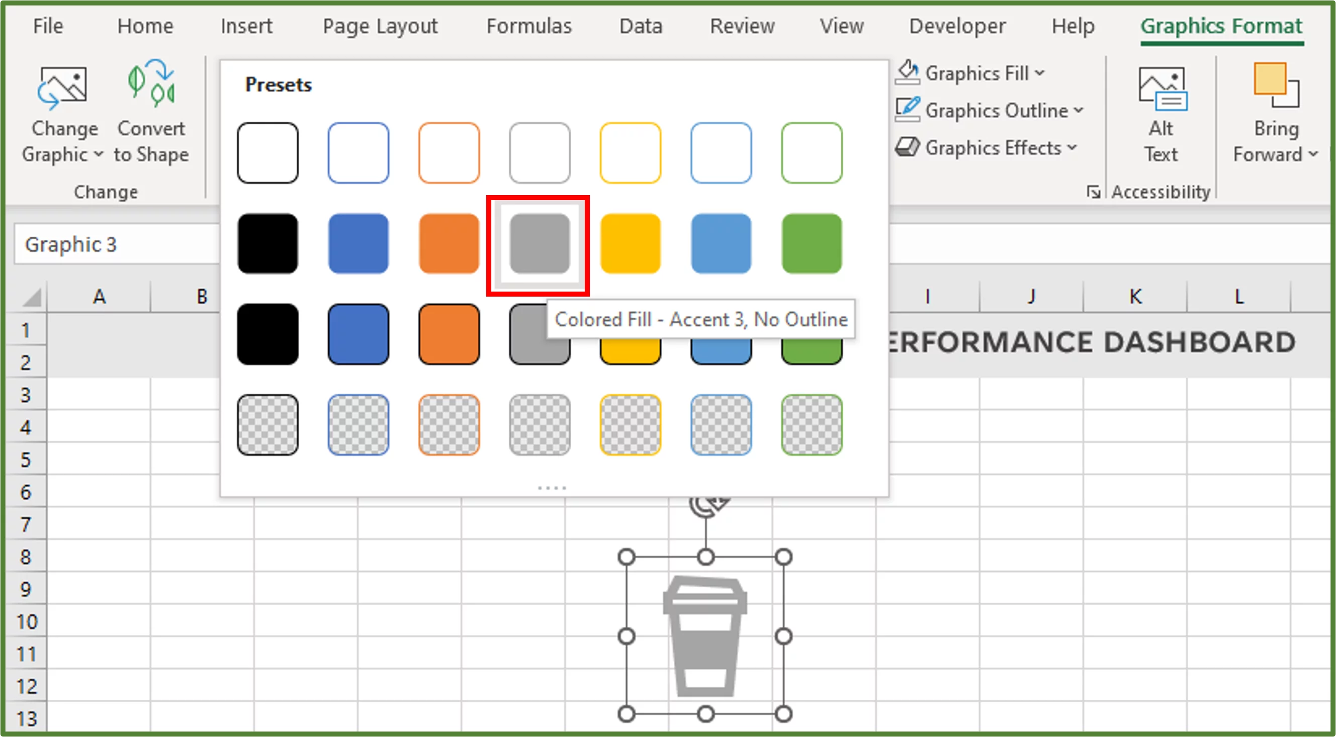
With the image selected, go to the Graphics Format Tab. In the Graphics Styles Group choose the Colored Fill – Accent 3, No Outline Preset.

 

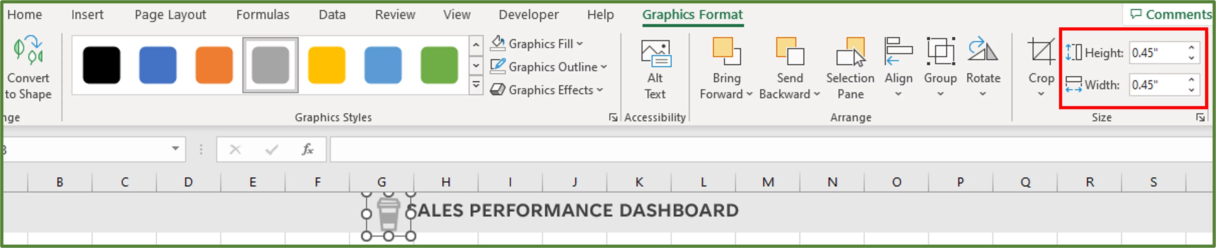
Resize the image to 0.45″ by 0.45″ and position it as shown below. Use the arrow keys on your keyboard, for more precise positioning.

 

Step 3

We will go back to our sheet called Data. Since we want to create a Table that will update automatically, when we add new rows. With one cell in the range selected, press CTRL-T on your keyboard to create a Table.

The Create Table Dialog Box should appear.

 

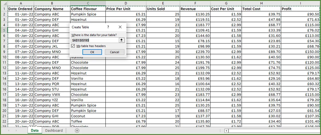
Click Ok.

 

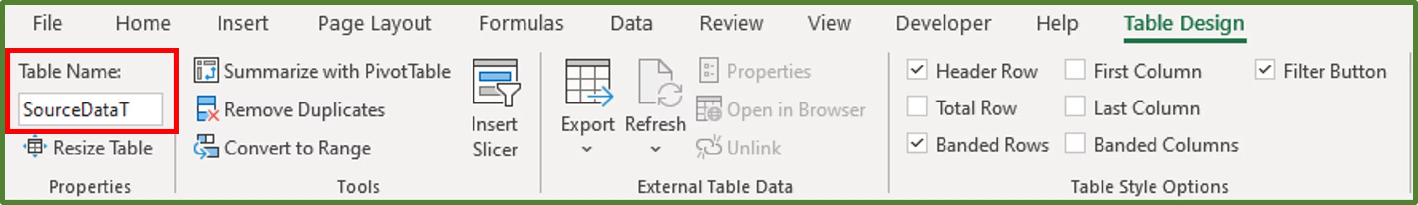
With one cell in the Table selected, go to the Table Design Tab. In the Properties Group change the name of the Table to SourceDataT.

 

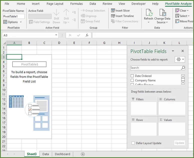
Select any cell in the Table and go to the Insert Tab. In the Tables Group, select the PivotTable option. Using the PivotTable from table or range Dialog Box, ensure New Worksheet is checked. Click Ok.

 

You should see the following.

 

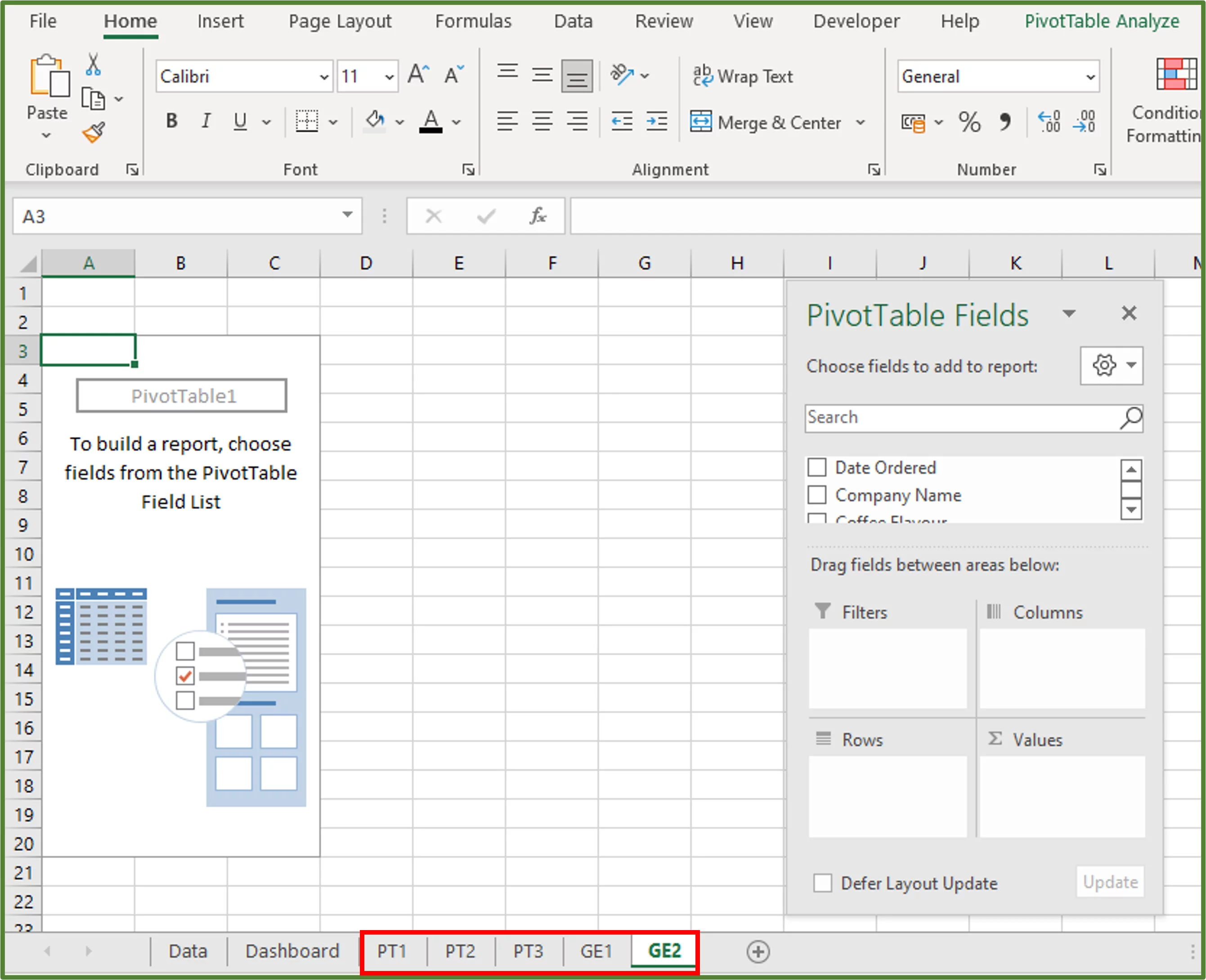
We need five PivotTables in total. Three for PivotChart creation and two for the graphical elements creation.

So make four copies of Sheet3, and name:

• • • • Sheet3 – PT1
      • The first copied sheet – PT2
      • The second copied sheet – PT3
      • The third copied sheet – GE1
      • The fourth copied sheet – GE2

 

Step 4

Now, we will add fields to our first PivotTable. We will then create a PivotChart by using this PivotTable.

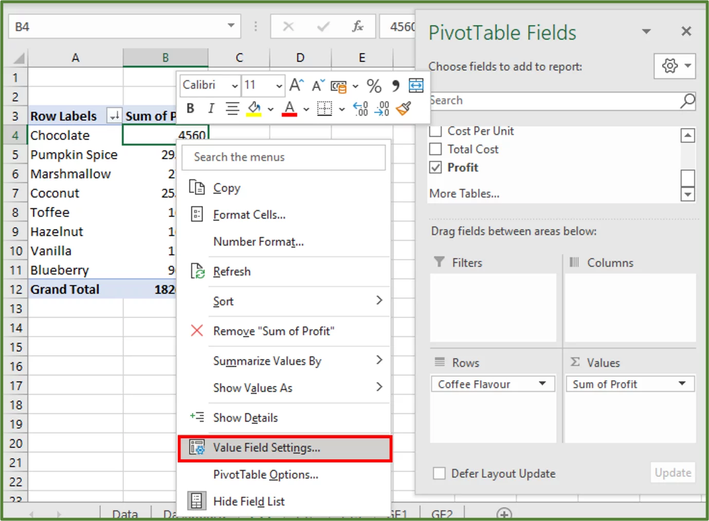
So go to the sheet called PT1.  We want to add the Coffee Flavour field to the Row Labels section and the Profit field to the Values section.

Using the PivotTable Fields Pane, right-click the Coffee Flavour field and choose the Add to Row Labels option. Right-click the Profit field and choose Add to Values.

 

We want to show the numbers in the Sum of Profit column, in the PivotTable as currency values. So, select any cell in this column and right-click and choose Value Field Settings…

 

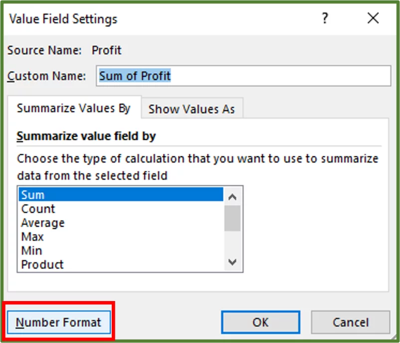
Using the Value Field Settings Dialog Box, select the Number Format option.

 

Using the Format Cells Dialog Box, select Currency. Set the decimal places to 0 and select the appropriate currency.

 

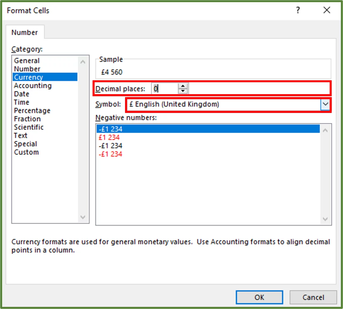
Click Ok and then Ok again.

 

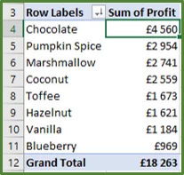
We can now insert the first PivotChart. We do this by selecting a cell in the PivotTable and then going to the PivotTable Analyze Tab. In the Tools Group, select the PivotChart option.

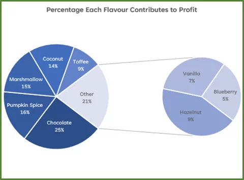
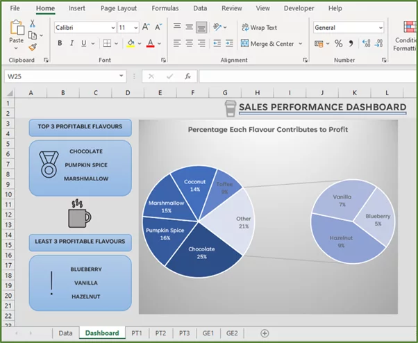
Using the Insert Chart Dialog Box, we select Pie. Then select the pie of pie option. Click Ok.

 

A Pie chart is useful when you want to show the contribution of each segment (slice) to the whole (pie).  If you have many slices, then a pie of pie chart is the most suitable type of option to use.

There are extra things on our PivotChart that are not needed, for our purposes. So, the first thing we would like to do, is hide all the field buttons on the chart and delete the legend.

To do this, right-click the Sum of Profit button on the chart and select the Hide All Field Buttons on Chart option. Then select the legend and press the Delete key on your keyboard.

Then select the current title Total on the chart. Change the text to Percentage Each Flavour Contributes to Profit.

 

With the title selected, go to the Home Tab. In the Font Group, change the font to Tenorite, the font size to 12, the weight to bold and the colour to Black, Text 1, Lighter 35%.

 

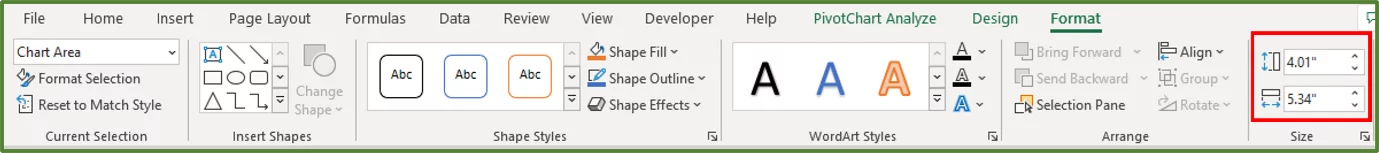
Select the chart and go to the Format Tab. In the Size Group, change the dimensions of the chart to 4.01” by 5.34”.

Now, increase the size of the plot area of the chart. Select the plot area and make it bigger as shown below.

 

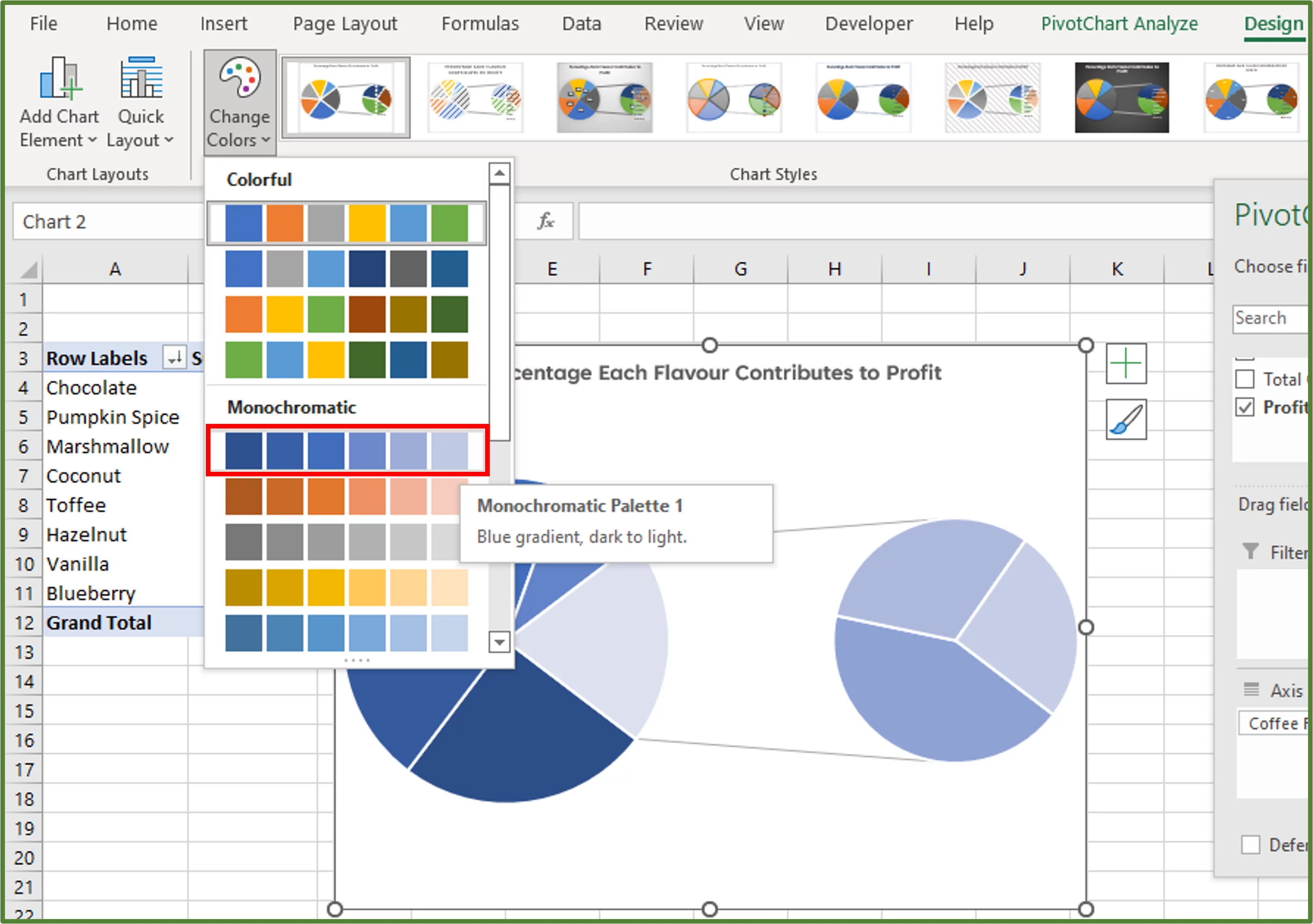
There are too many colours, on our chart that don’t fit into the desired colour scheme. To sort this out, we first have to select the chart.

With the chart selected, go to the Design Tab. In the Chart Styles Group, click on the Change Colors button. In the Monochromatic section, choose the Monochromatic Palette 1 option.

 

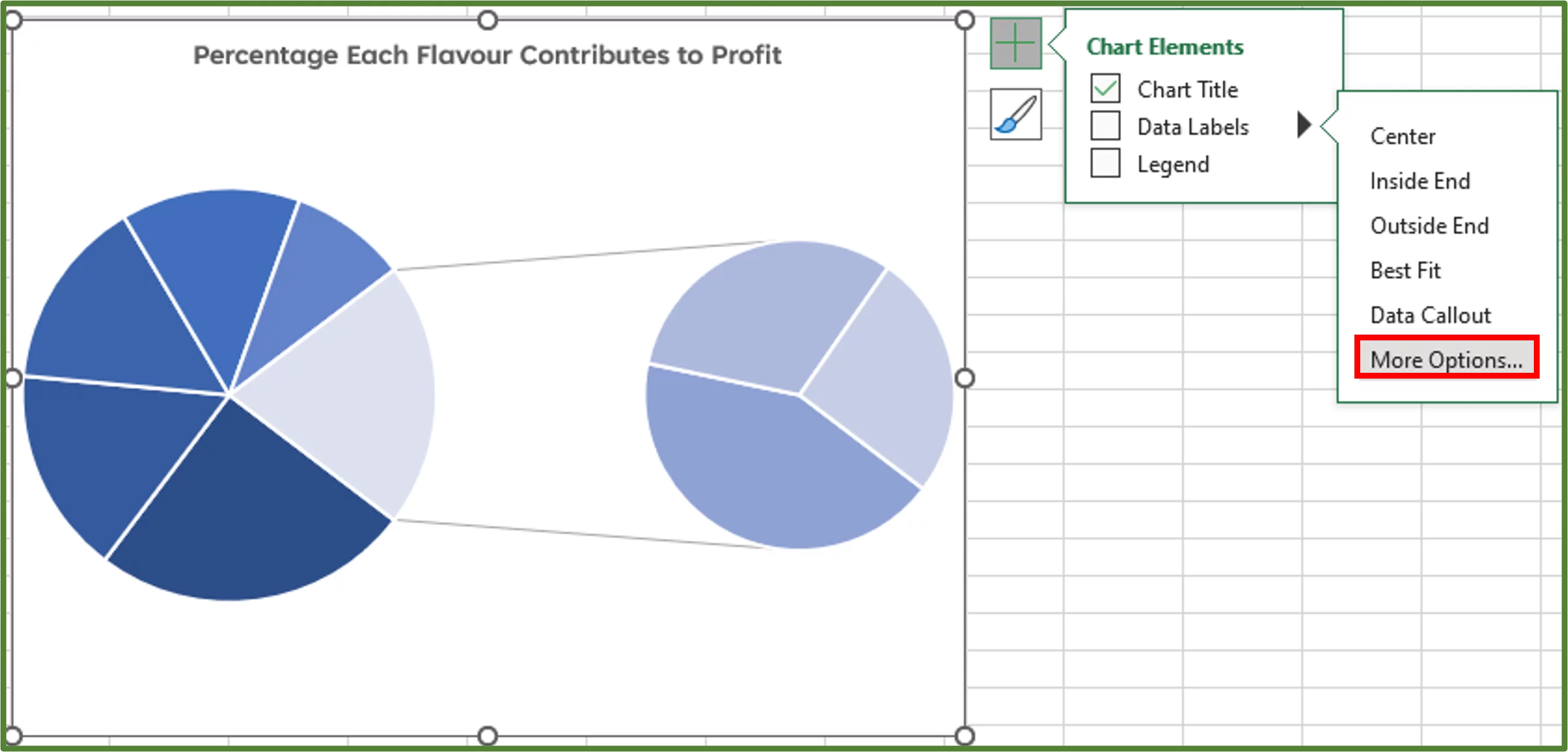
We now want to add and format the Data Labels. Select the chart and click on the Plus sign. Expand the Data Labels option and click on More Options…

 

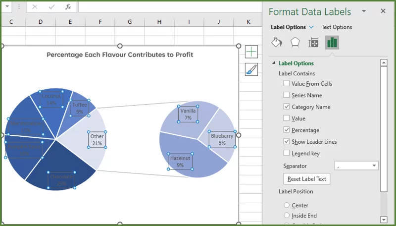
Using the Format Data Labels Pane, check Category Name and Percentage and uncheck Value.

 

Select all of the Data Labels, by clicking on one of them. With all of the Data Labels selected, go to the Home Tab and in the Font Group, change the font to Tenorite.

Click off the chart to deselect everything.

We want to change the font colour, of some of our Data Labels in the darker slices, to white.

Click on one Data Label to select all the Data Labels, then click on the Chocolate Data Label again to select it. So, we selected only Chocolate.

With only the Chocolate Data Label selected, go to the Home Tab. In the Font Group change the font colour to white and move the label shown in the next screenshot.

 

Change the font colour of all the other Data Labels in dark slices, in the same way. Then reposition the Data labels according to your preference.

 

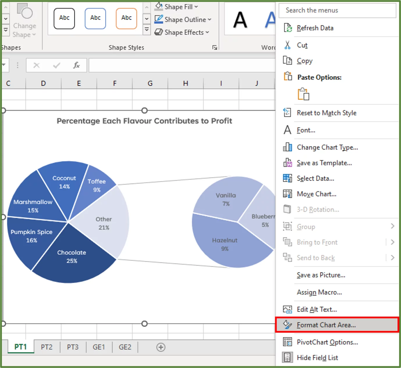
We have to change the background of the entire chart. To do this select the chart, right-click and choose Format Chart Area…

 

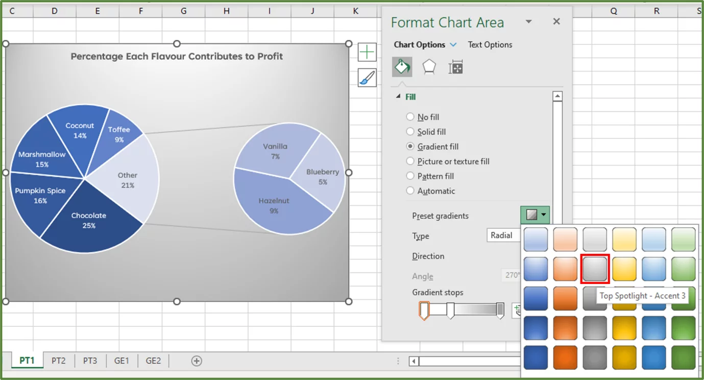
Using the Format Chart Area Pane, go to the Fill & Line section. Expand the Fill option and choose Gradient fill. Select the Top Spotlight – Accent 3 option.

 

Step 5

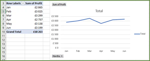
We will now create the next PivotTable we need. Go to the spreadsheet called PT2 and add the Date Ordered field to the Row Labels section.

 

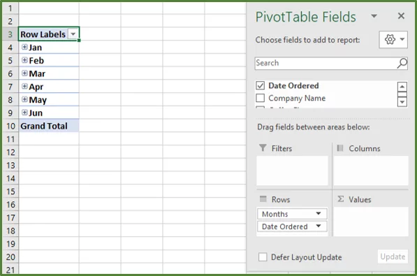
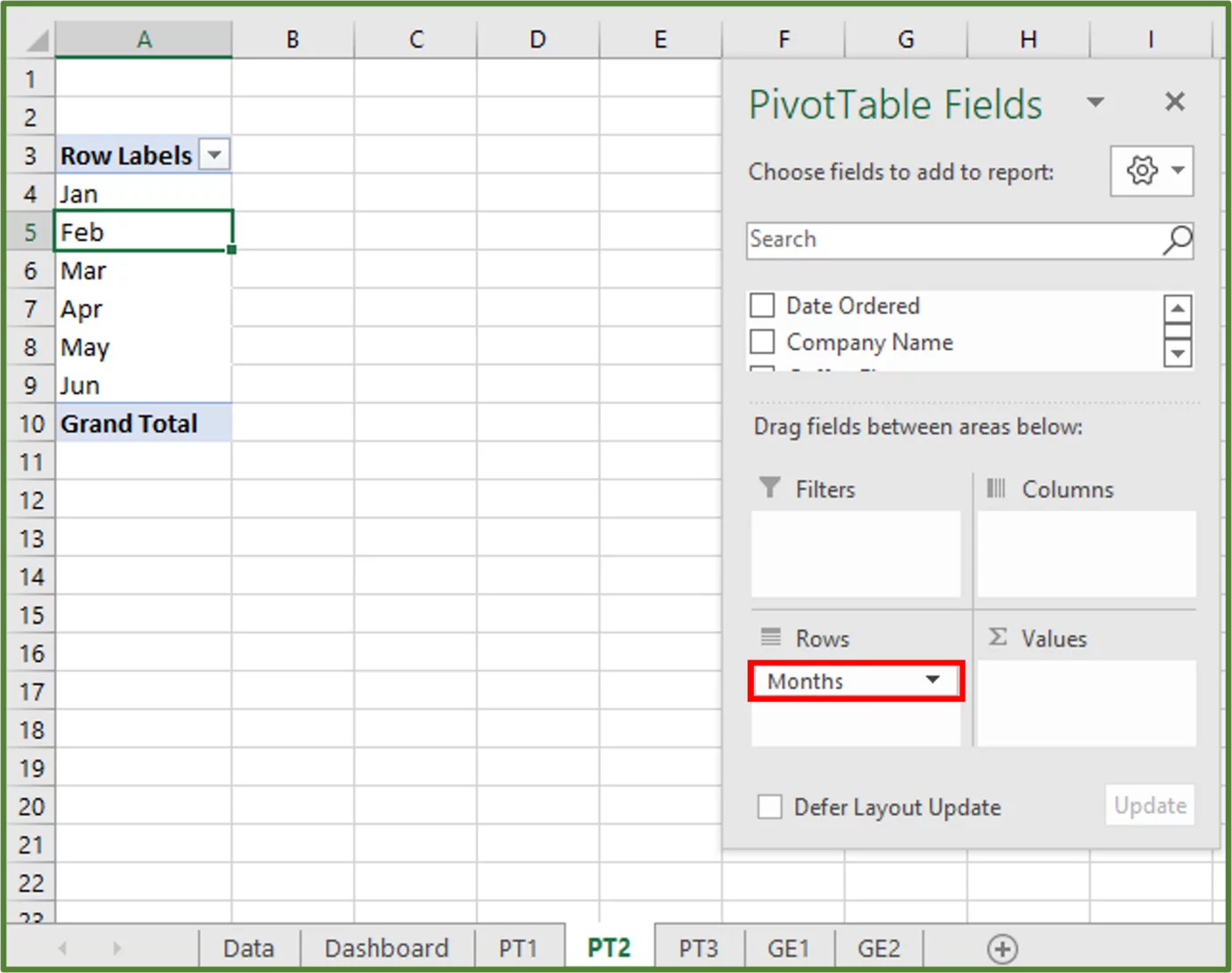
Click on the Date Ordered field, in the Row Labels section and select Remove Field. Since we only want to show Months.

 

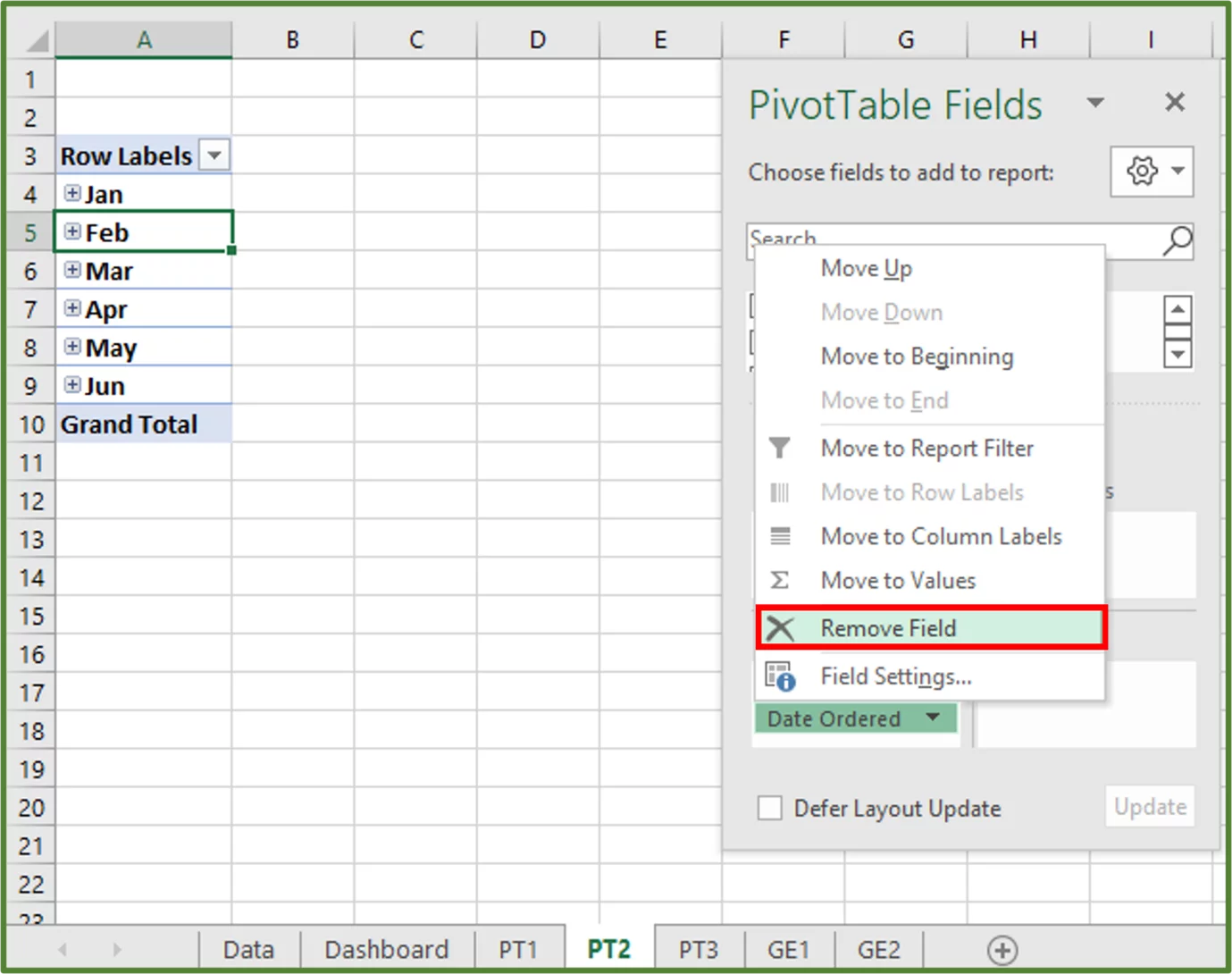
You should see the following.

 

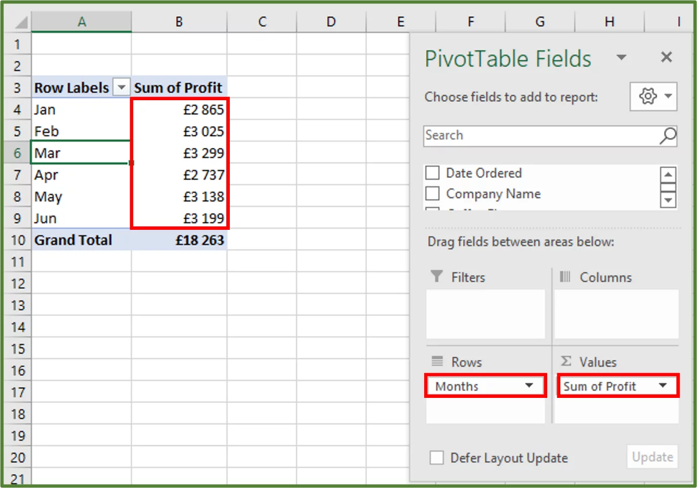
Add the Profit field to the Values section. Format the Sum of Profit Column to show currency with no decimal places.

 

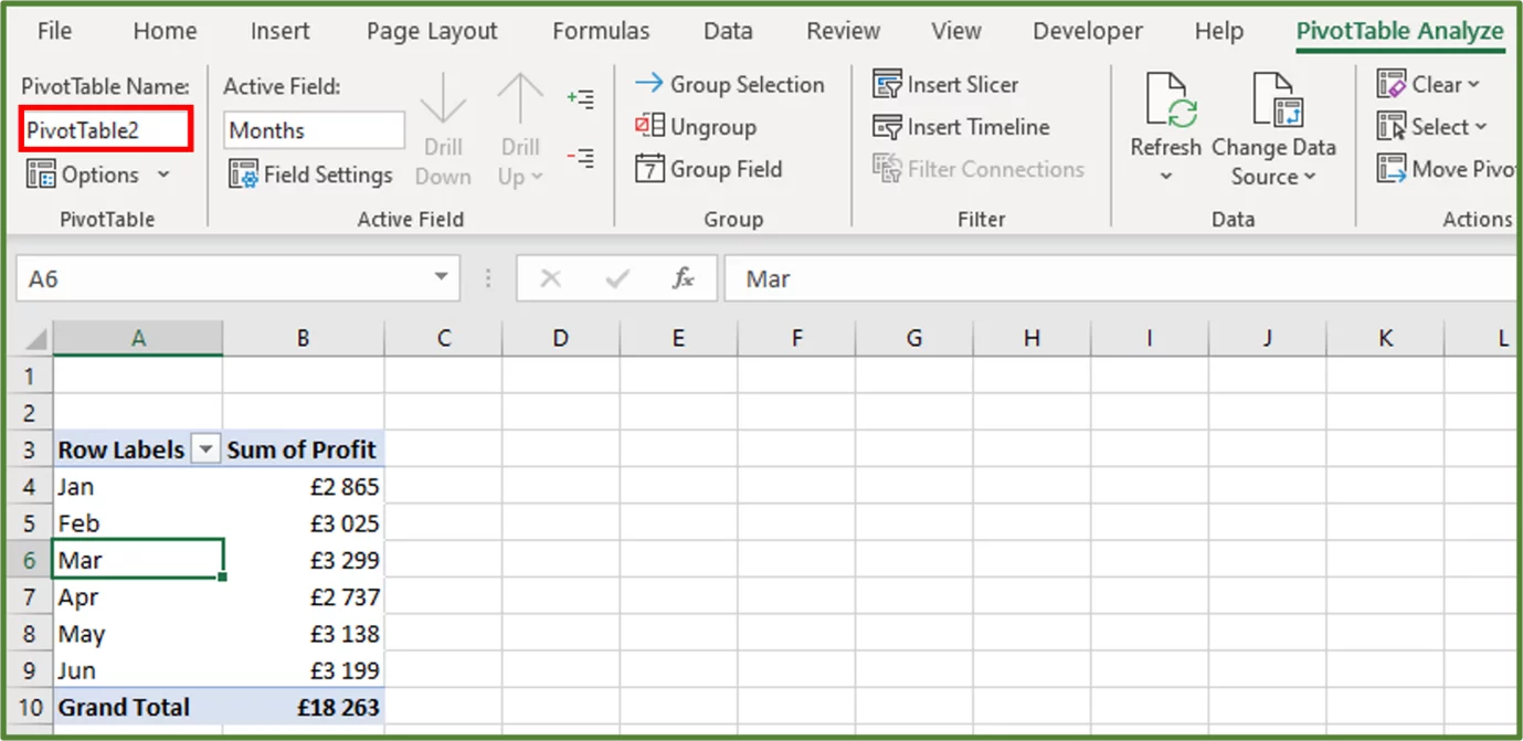
With one cell in the PivotTable selected, go to the PivotTableAnalyze Tab. In the PivotTable Group rename the PivotTable to PivotTable2.

 

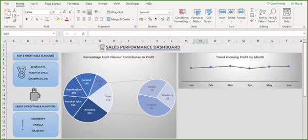
Go to the PivotTable Analyze Tab and in the Tools Group, select PivotChart. The Insert Chart Dialog Box should appear. Select Line and choose the first option. Click Ok.

 

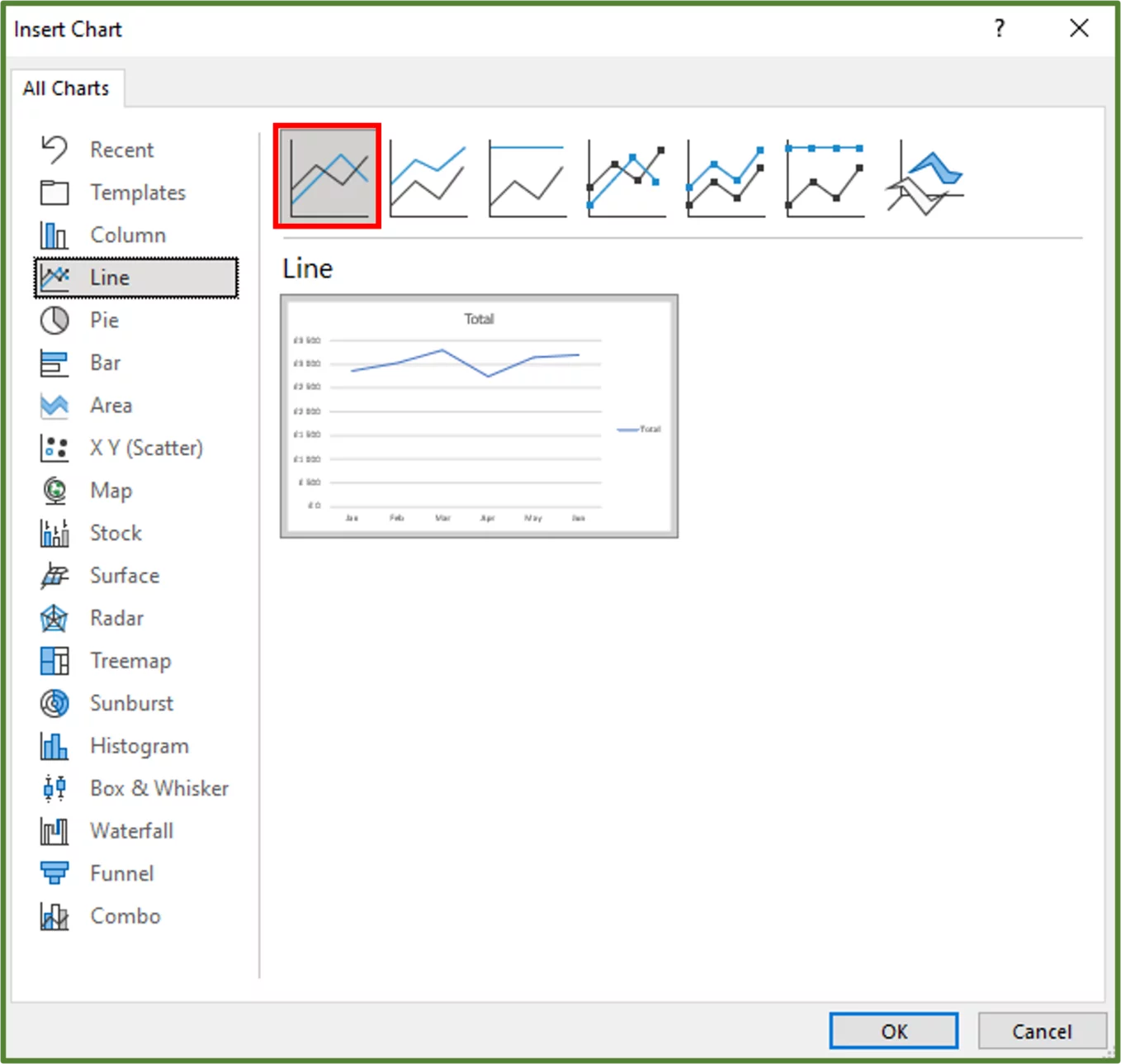
You should see the following.

Line charts are useful, when you need to show a trend over time. They are very simple and easy to understand.

Hide all the Field buttons on the chart. Delete the y-axis. You can delete the vertical axis by selecting it and then pressing the Delete key on the keyboard. In addition, delete the legend and the gridlines on the chart.

 

Select the markers, by clicking on one of the points where the lines meet.

 

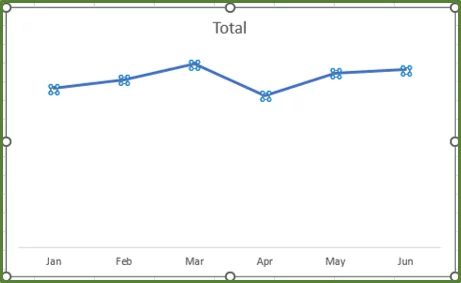
Right-click and choose Format Data Series.

 

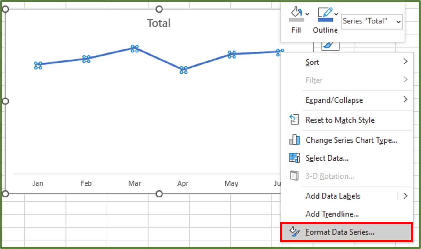
Using the Format Data Series Pane, select the Fill & Line option. Change the Line Colour to one of the grey colours. In this case we used Light Gray, Background 2, Darker 50%.

 

Using the Format Data Series Pane, select the Marker option. Expand the Marker Options section.  Choose the Built-in option. Select the circle type and set the size to 7.

 

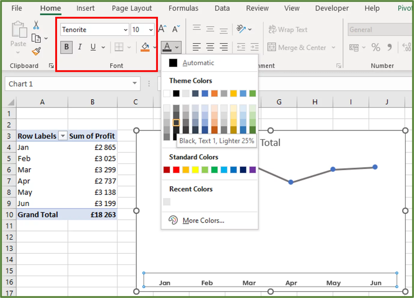
Select the horizontal axis by clicking on it. Change the font to Tenorite, the font size to 10, the font weight to bold. Change the font colour to Black, Text 1, Lighter 25%.

 

With the horizontal axis selected, go to the Format Tab.  In the Shape Styles Group, select the Shape Outline option.

Change the Outline colour to Black, Text 1, Lighter 25%. Set the Weight of the Outline to 1 ½ points. 

 

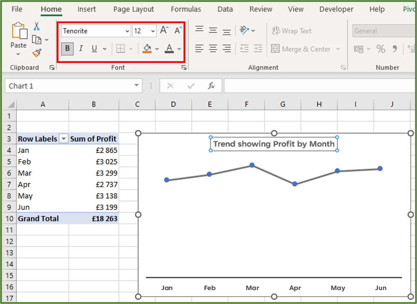
Change the title of the chart to Trend showing Profit by Month. Set the font to Tenorite, the font size to 12, the font weight to bold and the font colour to Black, Text 1, Lighter 35%.

 

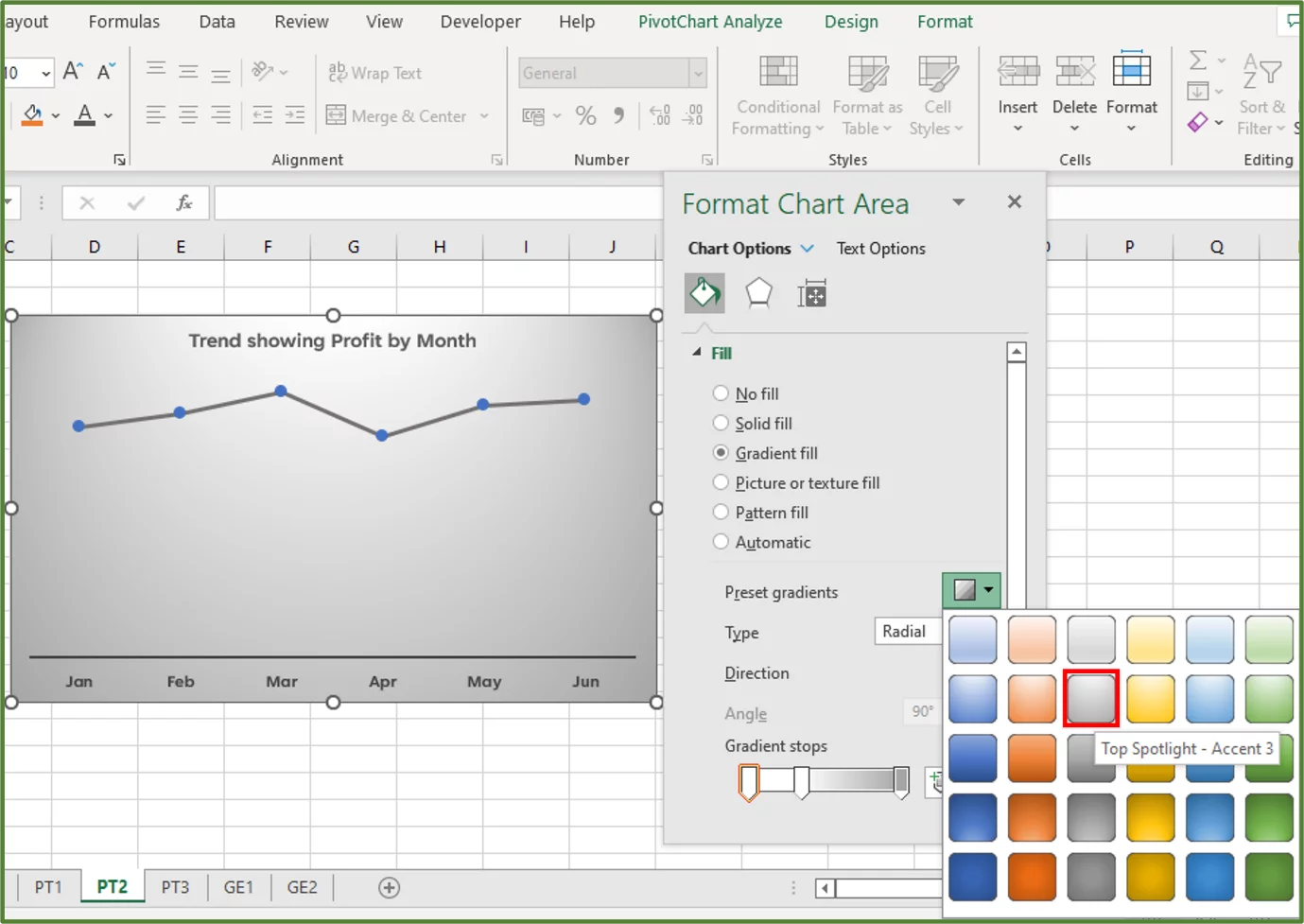
Select the chart. Right-click and choose Format Chart Area… The Format Chart Area Pane should appear. Expand the Fill options and choose Gradient fill. Choose the Top Spotlight – Accent 3 gradient fill.

 

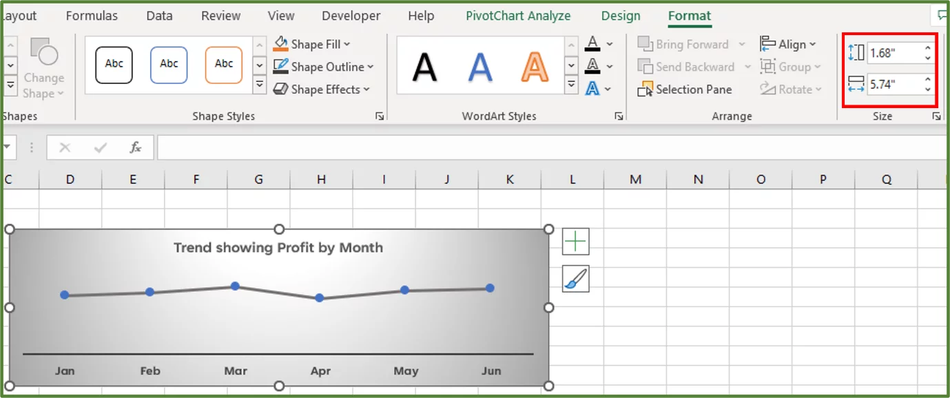
Select the chart and go to the Format Tab. In the Size Group set the dimensions of the chart to 1.68” by 5.74”.

 

Step 6

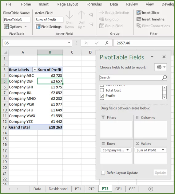
We will now create the next PivotTable that we need. Go to the spreadsheet called PT3.

Note: If your Field list is not showing for whatever reason, then click on one cell in the PivotTable. Go to the PivotTable Analyze Tab and in the Show Group, click on the Field List Button.

Rename the PivotTable to PivotTable3. Add Company Name to the Row Labels section and Profit to the Values Section. Format the Sum of Profit column to show currency with no decimal places.

 

With one cell in the PivotTable selected, go to the PivotTable Analyze Tab. In the Tools Group, select PivotChart.

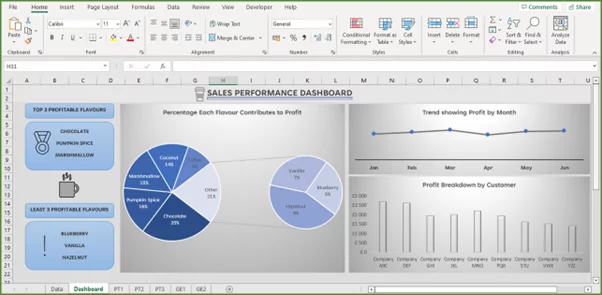
Choose Column and then select the Clustered Column option.

 

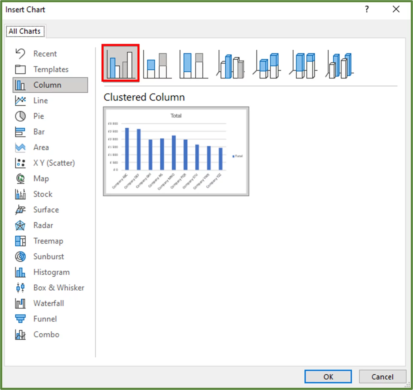
Click Ok.

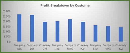
You should see the following.

 

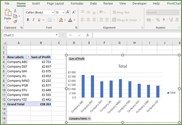
A Column chart is useful when you want to display data for each category in columns. This assists with comparative analysis.

Hide all the Field Buttons on the chart, delete the legend and the gridlines.

 

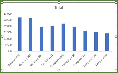
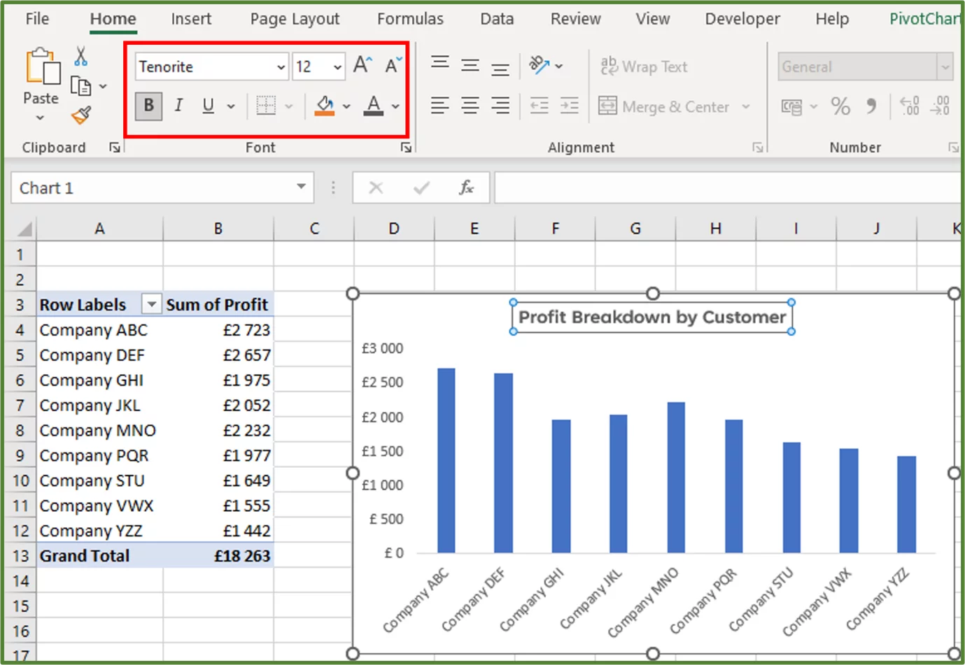
Change the title of the chart to Profit Breakdown by Customer. Set the font to Tenorite, the font size to 12, the font weight to bold and the font colour to Black, Text 1, Lighter 35%.

 

Change the background of the entire chart, to the gradient fill – Top Spotlight – Accent 3. Set the size of the chart to 2.29” by 5.74”.

 

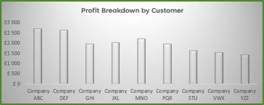
Select the data series, by clicking once on one of the blue columns. With the Data Series selected, go to the Format Tab. In the Shape Styles Group, change the Shape Fill to White, Background 1, Darker 15%.

 

With the Data Series still selected, go to the Format Tab. In the Shape Styles Group, select Shape Effects. Under Preset select Preset 8.

The result is the following.

 

Step 7

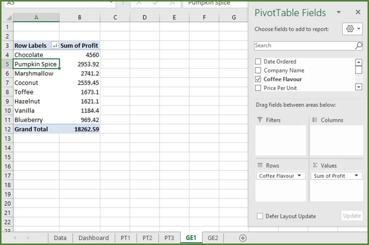
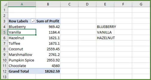
Let’s get started with creating part, of our first graphical element. Our first graphical element is going to showcase the top three most profitable flavours. Go to the sheet called GE1 and rename the PivotTable to PivotTable4.

Create a PivotTable with Coffee Flavour in the Row Labels section and Profit in the Values section. We then need to sort our Sum of Profit column, so that is it sorted from largest to smallest.

The result is the following.

 

We want to get the top three flavours in terms of profit, from the PivotTable.  Since we sorted the Sum of Profit Column from largest to smallest this is easy to do. Since these are the first three rows.

In cell E4 enter = UPPER(A4), in cell E5 enter = UPPER(A5) and in cell E6 enter = UPPER(A6).

 

In this way these cells will always return the top three flavours, in terms of profit.

So let’s look at creating the first part, of our second graphical element. Go to the sheet called GE2. We want our bottom three flavours in terms of profit generation, on this sheet.

Create a PivotTable with Coffee Flavour in the Row Labels Section and Profit in the Values section. This time sort from smallest to largest. Rename the PivotTable to PivotTable5.

In cell E4 enter = UPPER(A4), in cell E5 enter = UPPER(A5) and in cell E6 enter = UPPER(A6).

The result is the following.

Looking for a function to find data with? Read our guide on the XLOOKUP Function In Excel here!

Step 8

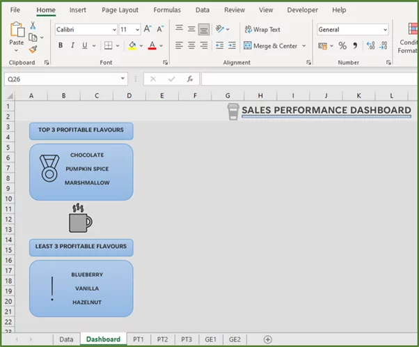
We are now going to start putting everything together. Return to the Dashboard sheet to complete the dashboard.

The first thing, we will do is select the range A3:U40 and fill it with this grey colour RGB(221,221,221).

 

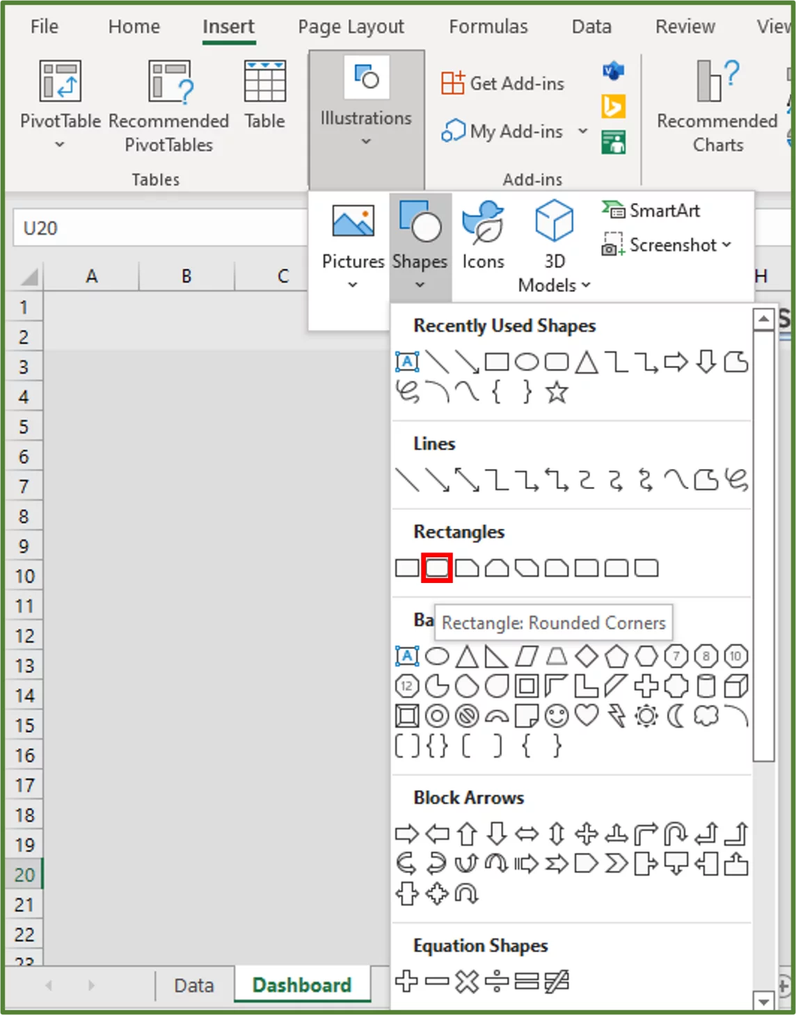
We want to create a decorative line underneath the text Sales Performance Dashboard. Go to the Insert Tab and in the Illustrations Group, choose Shapes. Select the standard Rectangle.

Draw the following rectangle underneath the Sales Performance text, the size should be 0.05” by 3.45” as shown below.

 

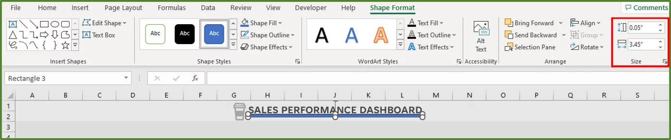
Note: You can zoom in when working with shapes and other graphics in order to see more clearly. The Zoom level is set to 120% for this step.

With the rectangle still selected, go to the Shape Format Tab. In the Shape Styles Group select Shape Effects. Choose Preset and then choose Preset 8.

 

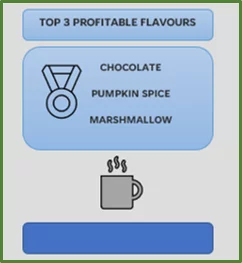
Let’s complete our first graphical element, which will showcase our top three most profitable coffee flavours on the Dashboard sheet. So, go to the Dashboard Sheet.

Go to the Insert Tab and in the Illustrations Group, select Shapes. This time choose the Rectangle with Rounded Corners.

 

You can set your Zoom level back to 100%.

Draw a rectangle on the sheet of size 0.34” by 2.1”.

 

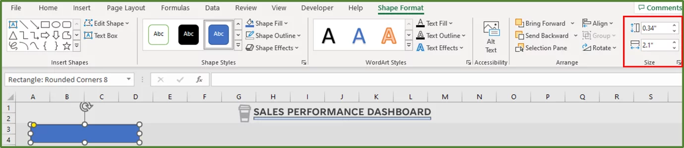
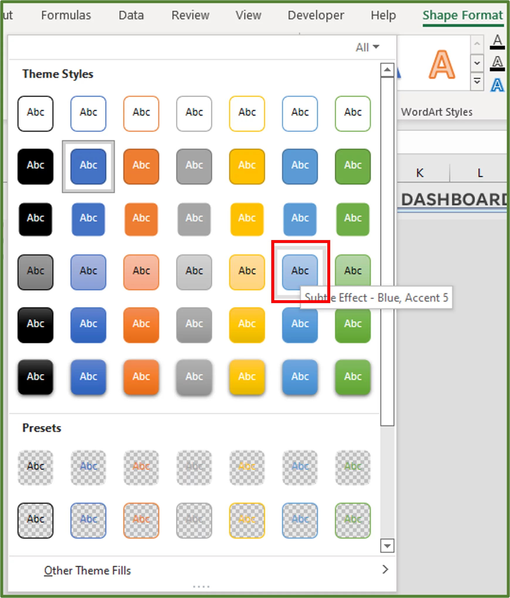
Select the rounded rectangle that we just created and go to the Shape Format Tab. In the Shape Styles Group, select the Subtle Effect – Blue, Accent 5 Theme Style.

 

With the rectangle still selected, go to the Home Tab. In the Font Group, change the font to Tenorite. Set the font size to 9.5, the font weight to bold, and the font colour to Black, Text 1, Lighter 15%. Top Align and Center Align.

Enter the text, Top 3 Profitable Flavours.

 

Create another rounded corner rectangle of dimensions 1.15” by 2.1”. With this rectangle selected, go to the Shape Format Tab. In the Shape Styles Group, select the Subtle Effect – Blue, Accent 5 Theme Style.

 

We want to align the left edges of both rectangles. So, we do this by selecting both. Click on the larger rectangle and then while holding the CTRL key, click on the smaller rectangle.

With both rectangles selected, go to the Shape Format Tab. In the Arrange Group, choose Align and then the Align Left option.

 

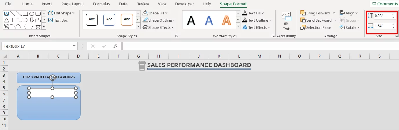
Now we want to insert a Text box on the second larger rounded corner rectangle. The size of the Text box should be 0.28” by 1.54”.

 

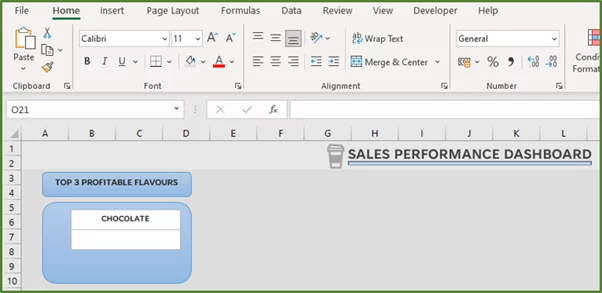
Select the Text box if you haven’t already.  In the Formula Bar type an = sign. Then go to the GE1 spreadsheet and select cell E4. Press Enter.

This means that the value in the Text box, will always display the value in cell E4 on sheet GE1.

 

With the Text box still selected, change the font to Tenorite, the size to 9, the font weight to bold. Change the font colour to Black, Text 1, Lighter 15%. Centre align the text.

Insert another Text box of size 0.28” by 1.54 and place it below the first Text box.

 

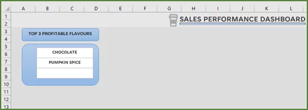
Select the second Text box and type an = sign in the Formula Bar. Then go to the GE1 sheet and select cell E5.

Press Enter. This means that the value in the second Text box will always display the value in cell E5 on sheet GE1.

With the second Text box still selected change the font to Tenorite, the size to 9, the font weight to bold. Change the font colour to Black, Text 1, Lighter 15%. Centre align the text.

Insert another textbox of size 0.28” by 1.54 and place it below the second textbox.

 

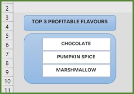
Select the third Text box and type an = sign in the Formula Bar. Then go to the GE1 sheet and select cell E6.

Then press Enter. This means that the value in the third Text box will always display the value in cell E6 on sheet GE1.

With the third Text box still selected change the font to Tenorite, the size to 9, the font weight to bold. Change the font colour to Black, Text 1, Lighter 15%. Centre align the text.

You should see the following.

 

Select all three Text boxes. You do this by selecting the first Text box, then while holding the SHIFT key, click on the second Text Box, then while still holding the SHIFT key, click on the third Text Box.

With all three Text boxes selected, go to the Shape Format Tab.  In the Shape Styles Group, in the Shape Fill option, choose No Fill. Then remove the outline.

 

We want to add a graphic that will emphasize the three most profitable flavours. Go to the Insert Tab and in the Illustrations Group, select the Pictures option. Choose Stock Images…

Select the Icons option and type Champion in the Search Box. Select the following image and click to Insert.

 

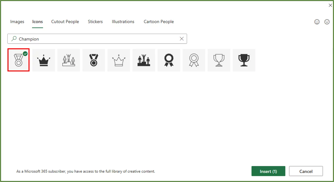
Resize the image by dragging the handles to make it smaller and place it in the position shown.

 

We want to insert another image now. Go to the Insert Tab and in the Illustrations Group, select Pictures. Choose the Stock Images…option.  Select Icons. Type Coffee in the Search Box and select this image.

Click to Insert.

 

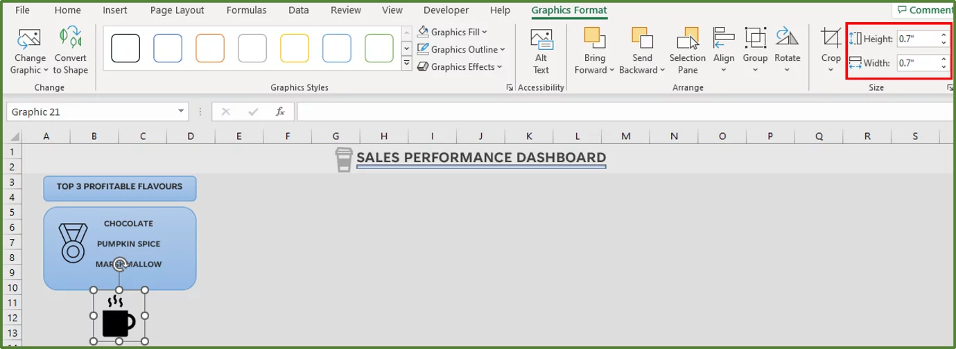
Resize the image to 0.7” by 0.7” and position it as shown below.

 

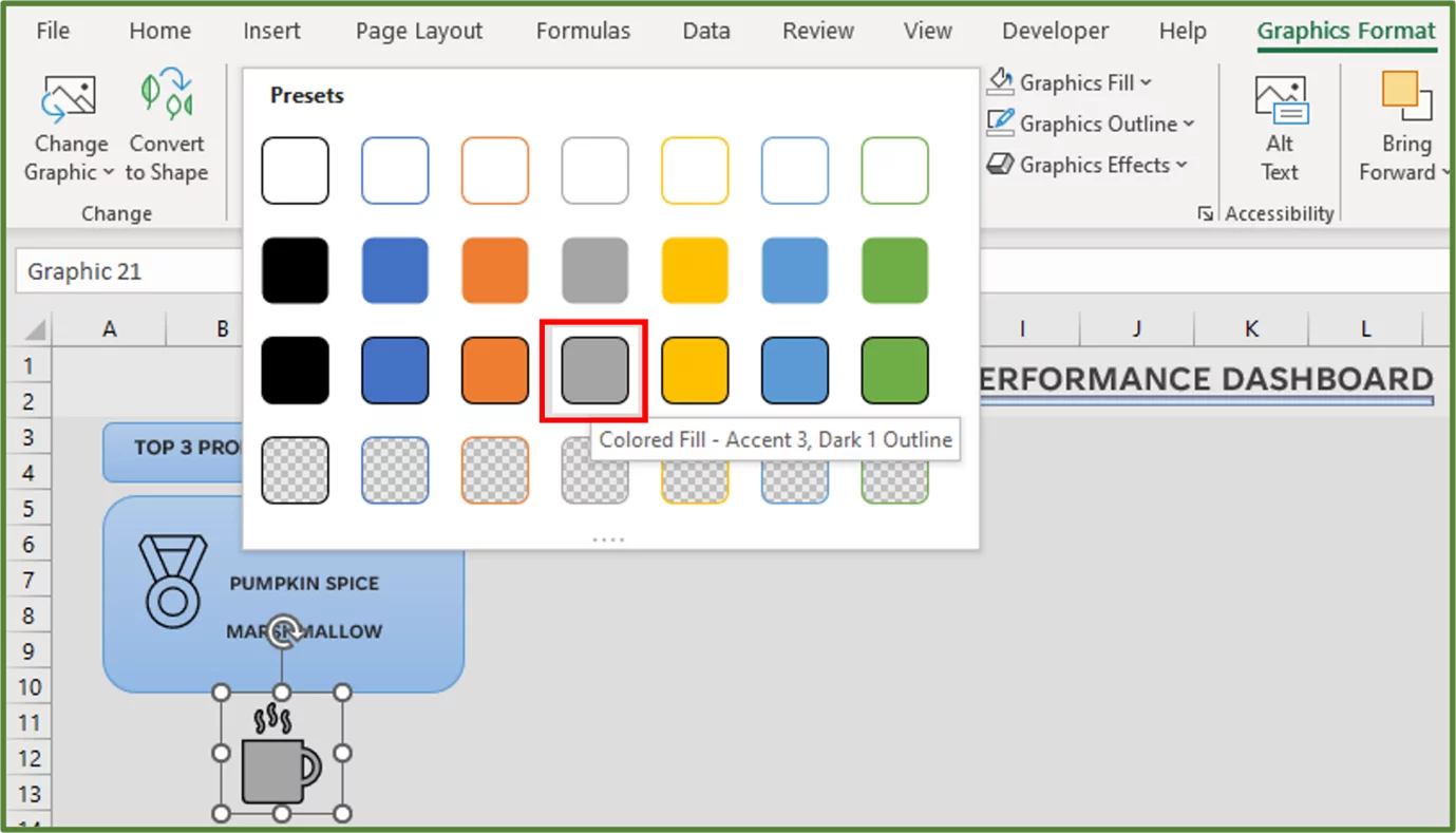
With the image still selected, go to the Graphics Format Tab. In the Graphics Styles Group, choose the Colored Fill – Accent 3, Dark 1 Outline preset.

 

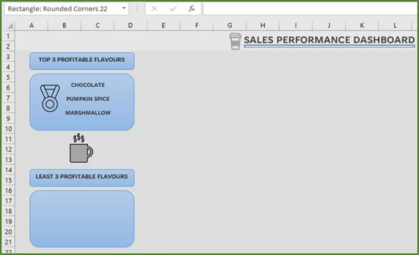
We now want to complete our second graphical element. Create a rounded corner rectangle of dimensions 0.34” by 2.1.

 

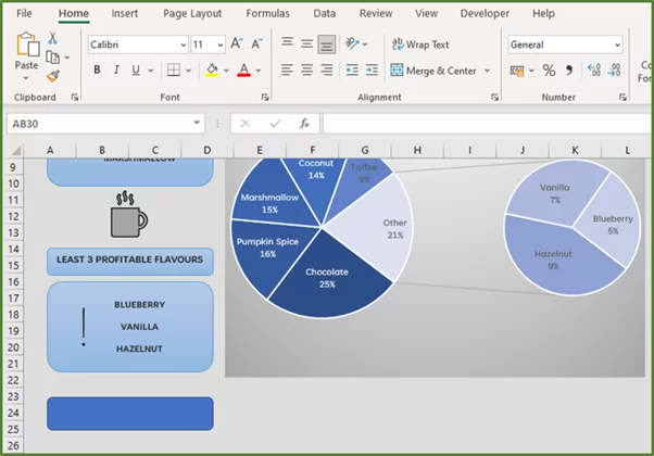
Now select the Top 3 Profitable Flavours rectangle and go to the Home Tab. In the Clipboard Group, select Format Painter and now click on the third rounded rectangle. This will change the format of the third rectangle to look like the first.

 

Now change the text in the third rounded corner rectangle to read Least 3 Profitable Flavours. Draw another rounded rectangle underneath the third one of dimensions 1.15” by 2.1”.

With this rectangle selected, go to the Shape Format Tab. In the Shape Styles Group, select the Subtle Effect – Blue, Accent 5 Theme Style.

 

Create three Text boxes on the fourth rounded corner rectangle. Ensure that the dimensions of all the Text boxes are 0.28” by 1.54.

• • • • Select the first Text box if you haven’t already.  In the Formula Bar type an = sign. Then go to the GE2 spreadsheet and select cell E4. Press Enter. This means that the value in the first Text box will always display the value in cell E4 on sheet GE2.

• • • • Select the second Text box.  In the Formula Bar type an = sign. Then go to the GE2 spreadsheet and select cell E5. Press Enter. This means that the value in the second Text box will always display the value in cell E5 on sheet GE2.

• • • • Select the third Text box.  In the Formula Bar type an = sign. Then go to the GE2 spreadsheet and select cell E6. Press Enter. This means that the value in the third Text box will always display the value in cell E6 on sheet GE2.

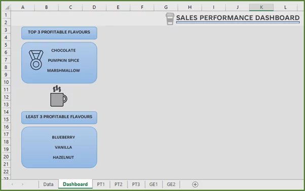
Ensure that the formatting of these Text boxes, is the same as the first three. You should see the following.

 

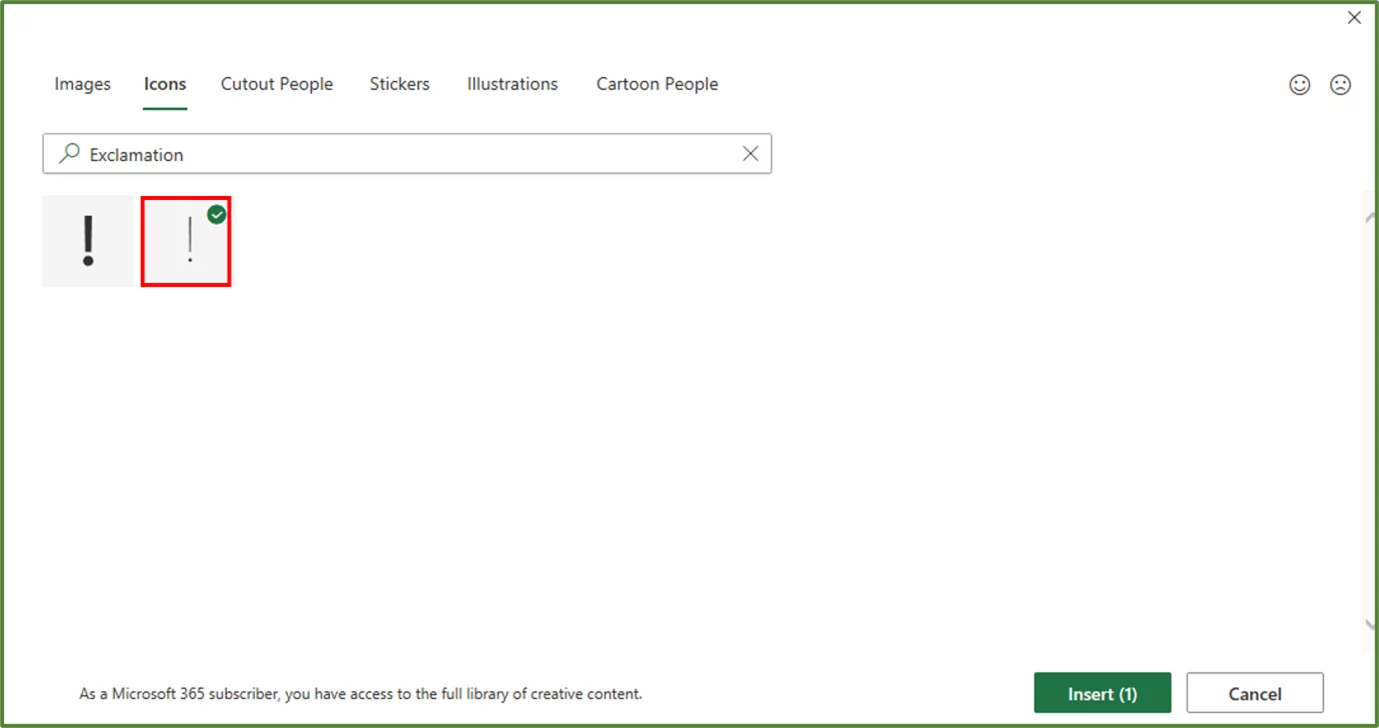
Go to the Insert Tab and in the Illustrations Group, select the Pictures option. Choose Stock Images…

Select the Icons option and type Exclamation in the Search Box. Select the following image and click to Insert.

 

Resize the image and position it as shown below.

 

Step 9

We will now add the needed charts to our Dashboard sheet. So go to sheet PT1 and cut and paste our pie of pie Pivot Chart to the Dashboard sheet. You can use the CTRL-X shortcut.

Use the Align options if you need to, in order to align the top of the chart to the top of the first rounded corner rectangle.

 

Go to sheet PT2 and do likewise for the Line chart. Position the PivotChart on the Dashboard sheet as shown below.

 

Go to sheet PT3 and do likewise for the Column chart. Position the PivotChart on the Dashboard sheet as shown below.

 

Step 10

Now we will look at adding interactivity to our dashboard.

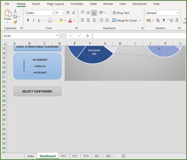
The first thing we have to do, however is add another rounded corner rectangle of size 0.42” by 2.1”. We will place it below the second graphical element.

Don’t worry about scrolling down – we will sort this out later, so that the end user won’t have to scroll down.

 

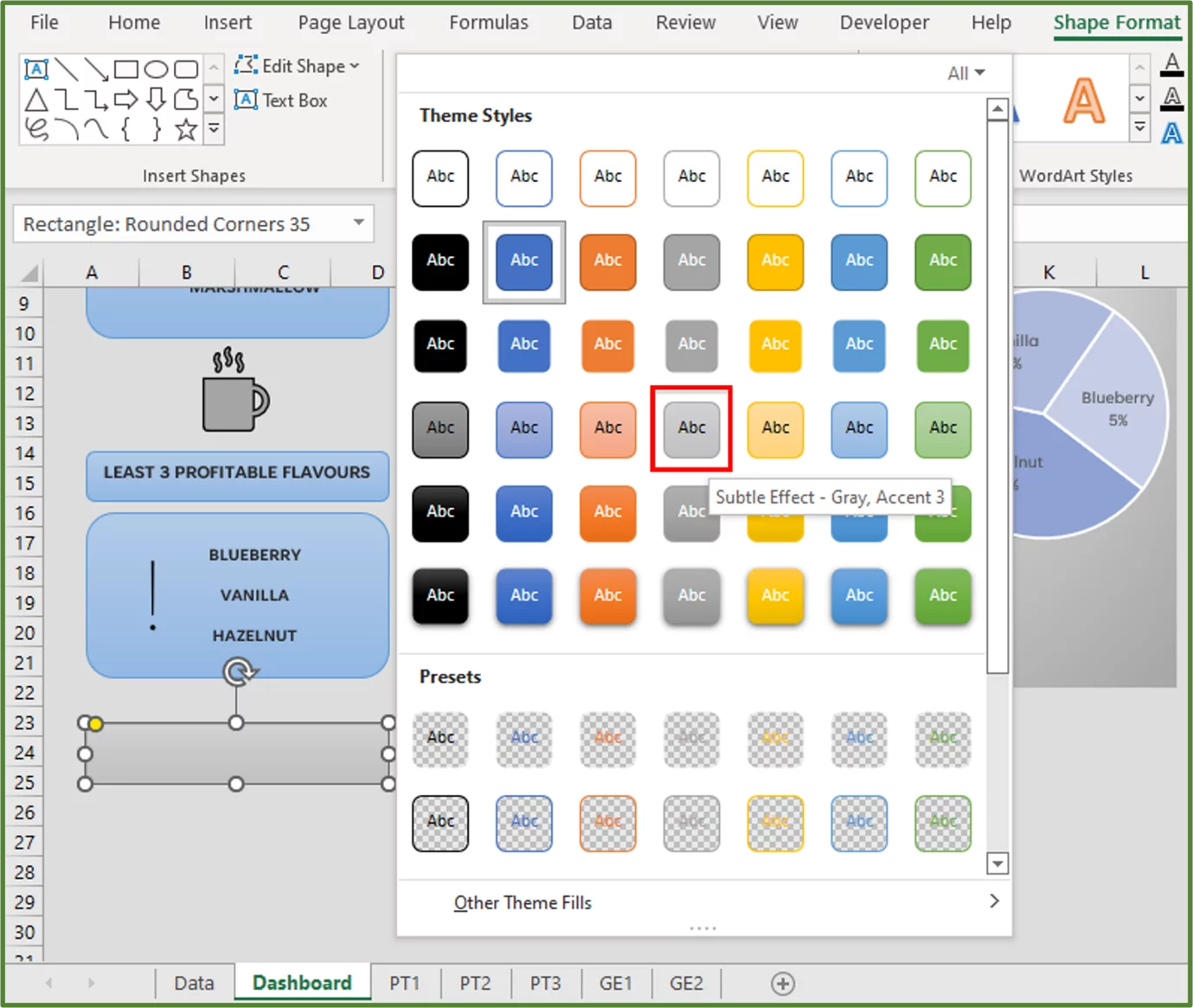
Select the rectangle. With the rectangle selected,  go to the Shape Format Tab. In the Shape Styles Group select the Subtle Effect – Gray, Accent 3 Theme Style.

 

Enter the text Select Customer:. Change the font to Tenorite and the font weight to bold. Ensure that the text is middle and centre aligned.

 

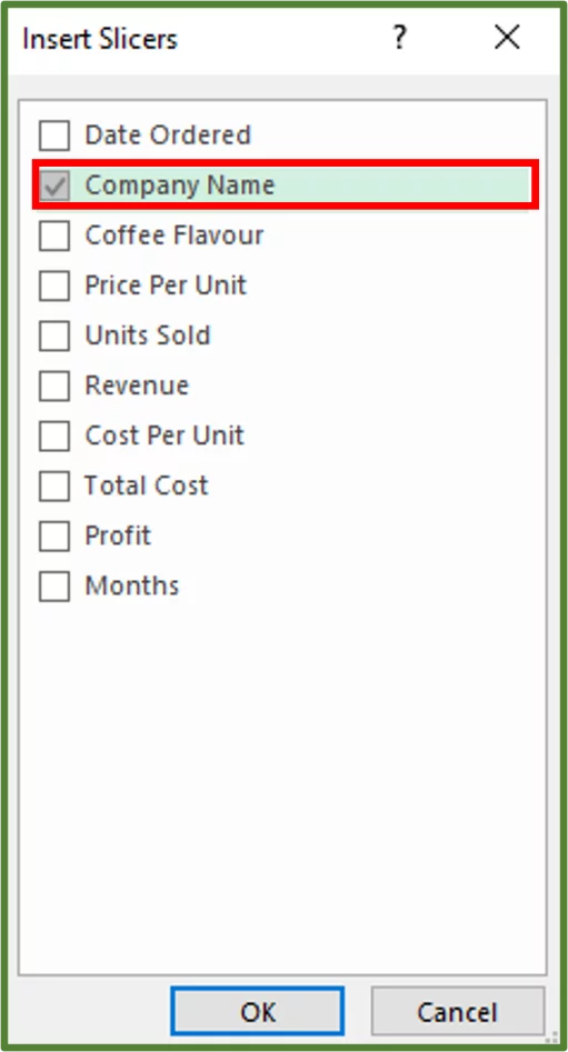
Now select the Line PivotChart. Go to the Insert Tab and in the Filters Group, select Slicer.

 

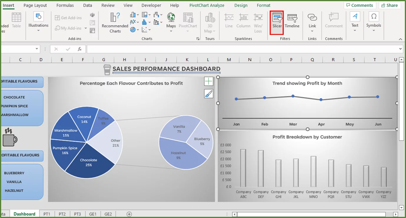
Using the Insert Slicers Window, select Company Name and then click Ok.

 

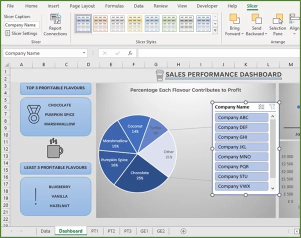
You should see the following.

 

Let’s look at formatting the Slicer.

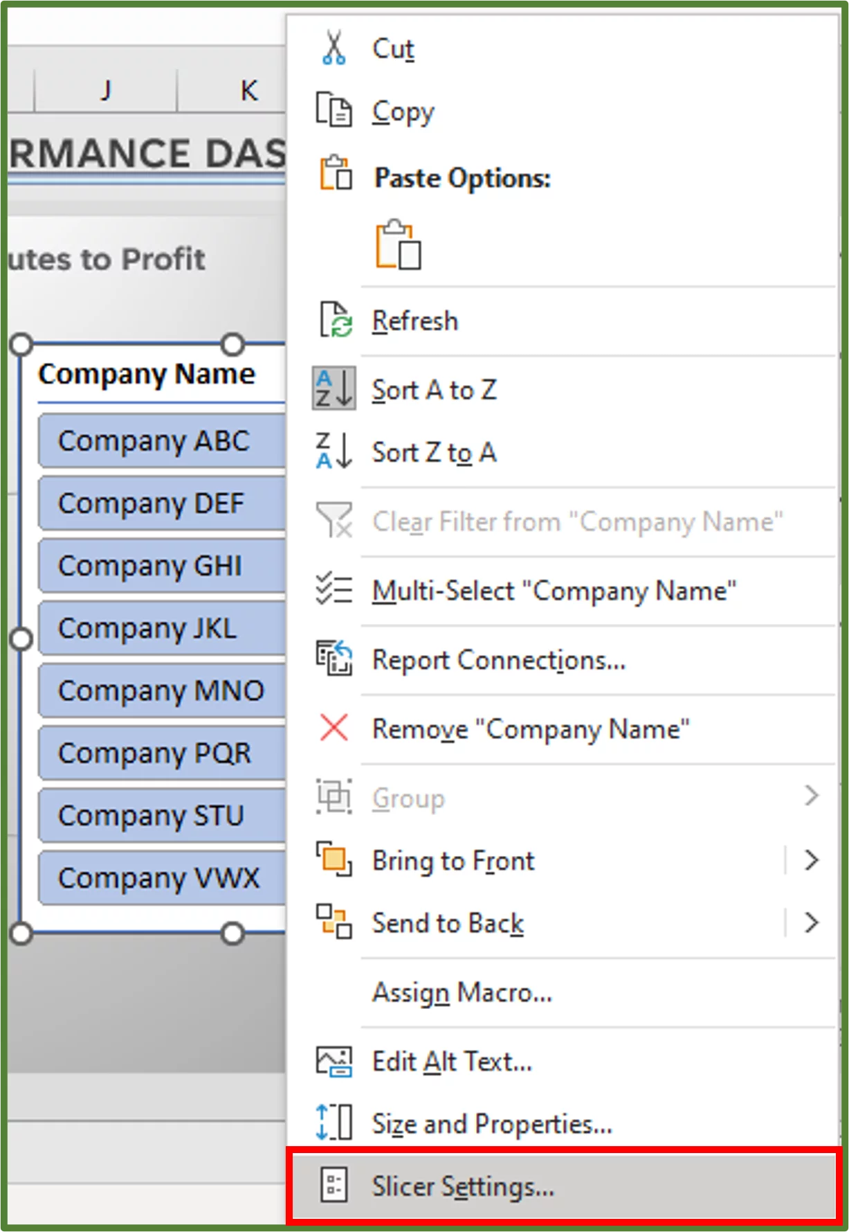
Right-click the Slicer and select Slicer Settings.

 

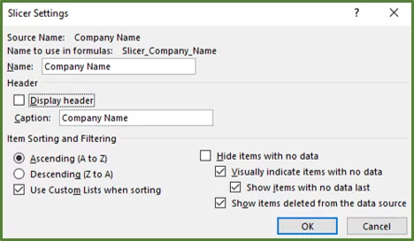
Uncheck Display header. Click Ok.

 

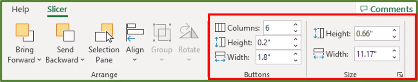
Select the Slicer. With the Slicer selected, go to the Slicer Tab. In the Buttons Group, change the number of columns to 6, the height to 0.2″ and the width to 1.8”.

While still in the Slicer Tab, in the Size Group change the Height to 0.66″ and the Width to 11.17″.

 

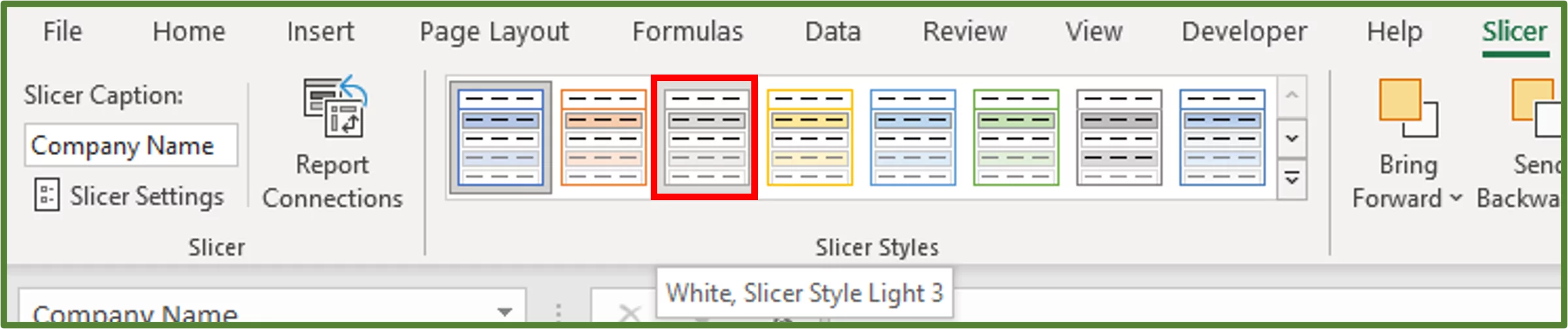
In the Slicer Tab, in the Slicer Styles Group, click on the White, Slicer Style 3 Light 3 option.

 

Move the Slicer into the position shown below. Align the bottoms of the Slicer and the rounded rectangle, if need be.

 

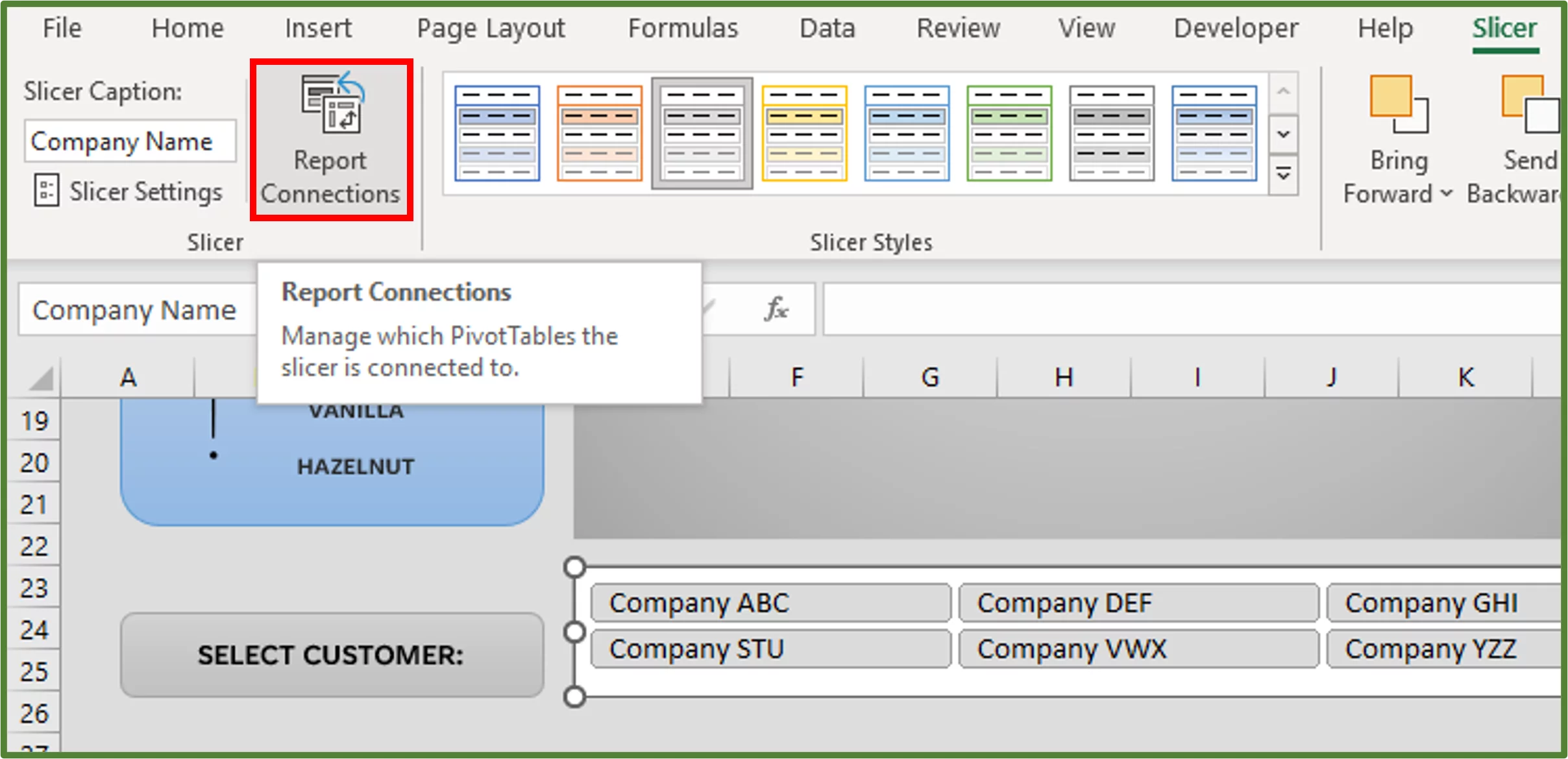
We now want to link the Column Chart to the Slicer as well. If we click on a button(s) on the Slicer currently only the Line chart will be filtered.

So select the Slicer and go to the Slicer Tab. In the Slicer Group, click on Report Connections.

 

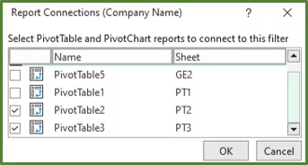
Check PivotTable2 and PivotTable3 only. Click Ok.

 

 

Hide all the other sheets, except the Dashboard sheet.

On the Dashboard sheet, go to the View Tab. In the Show Group, uncheck Gridlines, Headings and Formula Bar.

 

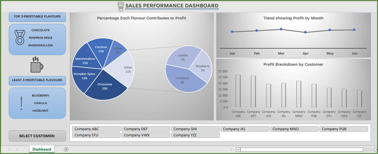
Now let’s see what happens, if we click a button on the Slicer. Let’s say the Company ABC button.  We will see the sales trend and the total profit generated from Company ABC.

 

Let’s say we want to see the combination of Company GHI and YZZ. We click on Company GHI, then holding down the CTRL key, we click on the other button to see the Line chart and the Column chart filtered accordingly.

 

To return our charts back to their unfiltered state. Select the Slicer and then press ALT-C on the keyboard.

 

Key insights

 

To learn more about Data Analysis in Excel, please read here!

Tip: You can add additional functionality to your Dashboard by using Form Controls such as scroll bars.

 

 

 

Conclusion

A dashboard is useful when you need to present KPIs in a visual format. Excel allows you to create professional dashboards that can be easily customized to your needs.

Looking for more Excel tips? Check out the UNIQUE Function in Excel article here!

Special thank you to Taryn Nefdt for collaborating on this article!

For more on Excel, check out our Using AI With Excel article here!