Creating Arrays – Excel Array Formulas

Array formulas are some of the most powerful functions in Excel.

But we often find on our courses that they are some of the hardest to understand!

That is one big reason why you’d often find Excel users resorting to time-worn, lengthy methods for performing even the simplest of Excel operations.

Mastering array formulas can help you save big on your time and energy.

They let you perform multiple calculations with ease.

38% of all Office Workers’ time is spent using Excel – optimising this time is important! For more Excel stats go here!

They are smartly designed and are very fruitful when it comes to complex operations.

Continue reading the article that follows to learn all about single-cell and multi-cell array formulas in Excel.

Arrays are a complex topic, which is why we only cover them on our advanced Excel courses.

What Is An Excel Array?

In literal terms, an array is defined as the ‘arrangement of a group of items’.

Specifically in Excel, an array is a collection of items populated together as a column or a row.

Array constants are a set of static values.

We all have created tons of arrays in Excel by populating individual cells.

However, an array can also be created through a multi-cell array formula and you’ll be amazed to know how.

For instance, we want to create an array in the shape of a row that consists of four names;

Tim, Brandon, Jonathon, and Taylor.

To do so, select the four cells where you want these names populated and write up a formula like the one below.

{“ Tim”, “Brandon”, “Jonathon”, “Taylor”}

Now! Wait. Don’t simply press enter. But bring three of your fingers to action to press Ctrl + Shift + Enter together. Take a look at the results.

Excel creates a row

There it is! You have just created an array in Excel. 
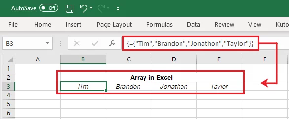
This is a horizontal array constant as it spreads across the columns. You may create a similar vertical array constant by selecting 4 rows instead of 4 columns before the formula is punched in.

Make sure you know which way you want your array constant to remain static!

Keep in mind that array constants never change when you copy a formula to other cells or values.

Attention!

The formula to be typed must be enclosed in curly brackets and not simple round brackets. Also, note how upon pressing Ctrl + Shift + Enter, Excel adds another pair of curly brackets to the formula.

The Excel array tools also enable the creation of Random arrays through the RANDARRAY function, which is one of Excels dynamic array functions.

What Is An Array Formula In Excel?

Simply put, an array formula in Excel is the one that allows you to perform multiple calculations in one go.

It evaluates individual operations within the formula and processes several values together to bring about the final result.

Not only that, but multiple-cell array formulas can also produce several values at a time.

That means array formulas can not only process several values but can also produce a range of values.

Within Excel, array formulas are created through the concurrent operation of the following three keys:

Ctrl + Shift + Enter

Excel denotes an array formula through flower or curly brackets added to the beginning and end of the formula.

These brackets are added as soon as you press Ctrl + Shift + Enter and can be seen through the formula bar (press F2).

Learn more about other Excel array tools such as the FILTER function here.

Did you know?

Array formulas that work under the operation of Ctrl + Shift + Enter are also known as CSE formulas (abbreviated for Ctrl + Shift + Enter).

Want to learn more about mathematics in Excel? Read our guide here all about Percentages in Excel.

Points to Note:

For array formulas, there are a few points that you must note:

      • These curly brackets only come through the concurrent operation of Ctrl + Shift + Enter. 
      • Editing the formula would turn it back into a regular formula unless you again hit Ctrl + Shift + Enter after you’re done editing.

When Should You Use Array Formulas In Excel?

Array Formulas in Excel are the most useful when you have lengthy datasets to your plate.

For example, take a look at the image below.

Quantity and sale price of different products for different customer orders

The above image represents the data of different customer orders with the quantity and sale price for products ordered by each customer.

How do you calculate the sales for March 202X?

Simple math, multiply the quantity and sales price for each product. Continue this step for each product ordered by each customer.

Add up these sub-totals to reach the final value for each customer order. Then add the total of each customer order.

Not to undercount, these are no less than 4 steps to be performed.

Also, the complexity keeps on adding as the number of products increases or as the data grows in size.

The old basic way of finding the total sales for March 202X is as follows.

Adding a column of sub-totals for each customer order

In the above image, we have included a new column for sub-totals where we have first found the total bill for each customer order.

And using the ‘Drag and Fill’ button, the same is calculated for other cells in the column.

Adding up the sub-totals for each customer order

Next, we have again constructed a new SUM formula for computing the total of all the sales made to each customer.

The above lengthy process can be simplified through one single array formula. Compose the formula as given below.

=SUM(B4:B10*C4:C10)*(D4:D10*E4:E10)

  • (B4:B10*C4:C10) is used to compute the total sales of Product A.
  • (D4:D10*E4:E10) is used to compute the total sales of Product B.
  • The SUM function is used to add up both the above sales.

After the above formula is composed, don’t just hit enter, but use:

Ctrl + Shift + Enter

This converts the above formula into a single array formula. And here are the results.

Excel computes the total sales for March 202X

Viola! No additional sub-total columns are required.

It takes only a single formula for Excel to compute the total sales for March 202X in one go.

Pro Tip: Note how excel has added curly brackets to the start and end of the formula to denote a single array formula.

Power Points of the Array Formula:

      • The modern-day array formula saves users’ time as you can cut down on unnecessary keystrokes for sub-totals.
      • Array Formulas come up as the handiest tool to replace tens of formulas with a single formula.
      • With single array formulas, Excel stores the intermediate results in its memory and so, you don’t need additional columns that make your data clumsy.

Another powerful tool from the Excel Array tools Library is the UNIQUE function. Learn about it here.

How To Use An Array Formula In Excel – Simple Example

Entering an array formula in Excel is all about three concurrent keystrokes.

Ctrl + Shift + Enter

Let’s put that together through an example.

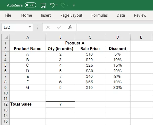
The image below represents the sale details for different products.

These details include the quantity, sale price, and discount offered per product.

We want to find the net sales (net of discount) for the month.
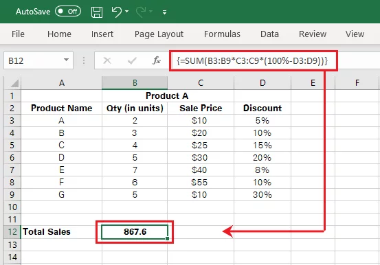
Sale, quantity, and discount data for different products

Can this be done in one go without us having to introduce multiple new columns for sub-totals and discount values? The array formula can help.

With array formulas, all the process is encapsulated within a single step by composing the right formula and feeding it through the three magic keys mentioned above.

Simply activate the cell against the total sales and set up the formula as follows.

=SUM(B3:B9*C3:C9*(100%-D3:D9))

Breakup of the formula:

    • The cell range B3:B9 consists of the quantity of each product ordered during the period under calculation.
    • This range is multiplied by the cell range C3:C9 which consists of the sale price of each product.
    • Another multiplication factor is added in the parenthesis for the computation of the discount. To find net sales, we must reduce the sales of each product (quantity * sale price) by the discount per product.
    • The cell range G3:G9 consists of the discount rate per product. (100%-D3:D9) is to reduce the discount from the sale.

The formula is all constructed. However, do not hit only ‘Enter’ but ‘Ctrl + Shift + Enter’.

Doing so, here are the results shown in Excel.

Excel computes the total net sales


Do not forget to take note of the curly brackets added by Excel to the opening and closing of the formula – this indicates that the enclosed formula is a single array formula and not a regular formula.

Multi-Cell Array Formulas

You must have enjoyed learning about the single-cell array formula in Excel. But what comes next is going to take you by surprise.

What is a Multi-cell array formula and how does it work?

A multi-cell array formula is where the formula and results of the array formula are spilled across a range of selected cells.

The formula is composed the same way as that of a single-cell array formula.

However, to have the results spread across a range of cells, all of those cells must be selected before the formula is composed and the CSE keys are used.

How is a single-cell array formula different from a multi-cell array formula?

Array formulas are designed to produce two kinds of results.

    • An array formula that covers a range of cells and the result spills into multiple cells is known as the multi-cell array formula.
    • An array formula where the formula and result are confined to a single cell is known as the single-cell array formula.

As seen above, with the single-cell array formula, we were able to perform operations with several calculations in one go.

However, if you want these calculations to be performed individually with results populated across a row/column, the multi-cell array formula is what you need.

Examples:

The below example must help you learn the primary difference between single-cell and multi-cell array formulas that is attributable to the selection of cell range.

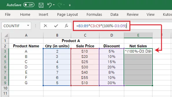
Continuing with the example above, let’s reiterate the source data for finding net sales.

Data for quantity, sale price, and discount per product

There are two ways how you can find the net sales in the above example, each of which is discussed below.

      1. Single-cell array formula:

A single-cell array formula is only to be used if you want the total net sales for all the products added up. To do so, activate a cell, and write in the following formula:

=SUM(B3:B9*C3:C9*(100%-D3:D9))

Hit Ctrl + Shift + Enter to have the single-cell results as shown below.

Excel computes the total net sales under one cell

$867.7 are the total sales net of discount for the period under calculation.

2. Multi-cell array formula:

A multi-cell array formula is to be used when you want a range of results i.e. net sales against each product.

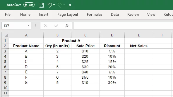
With a multi-cell array formula, you can find the net sales for each product only by composing a single formula.

However, what differentiates it from the single-cell array formula is the selection of cell range.

To enter the following formula, select cells E3:E9 where the net sales against each product are to be populated.

=(B3:B9*C3:C9*(100%-D3:D9))

Desired range selected and formula entered

Press Ctrl + Shift + Enter to yield the results shown below:
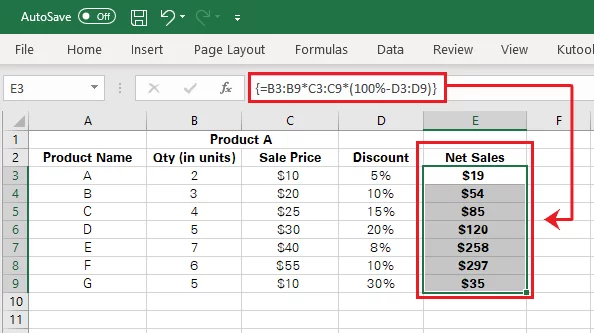
Excel computes the net sales against each product

The multi-cell array formula helps you find the range of net sales of each product in contradiction to the total sales computed by the single-cell array formula.

The SORT and SORTBY functions from the Excel array tool library can be used to sort data. Learn all about them here.

Conclusion

Excel array functions are incredible functions of the modern-day Excel.

The simple way they enable you to perform multiple calculations all at once is invaluable.

However, unfortunate to say, this function is also one of the most intimidating functions for many Excel users.

The reason for this lies in lack of practice more than in the complexity of the function.

Go ahead and practice the array formula with this knowledge and master it in no time! Interested in knowing some Excel Statistics? Hop here.

About Ben Richardson

Ben is a director of Acuity Training which he has been running for over 10 years.


He is a Natural Sciences graduate from the University of Cambridge and a qualified accountant with the ICAEW.


He previously worked as a venture capitalist and banker and so had extensive experience with Excel from building financial models before moving to learn SQL, Microsoft Power BI and other technologies more recently.