The RANDARRAY Function – Master Excel Array Tools!

While Excel already had RAND and RANDBETWEEN functions, what was the need for another random number generating function?

The RANDARRAY function was needed as it is not a mere random number generator but far more advanced and powerful. It allows users to specify the minimum and maximum values, the number of rows and columns, and whether the results should be in decimals or integers.

Details of this modern function are given below. More of our Excel course offerings are available here.

Did you know Only 48% of people have ever received any formal Excel training? Put yourself above the average candidate by attending our courses! For more Excel stats, read here!

Excel RANDARRAY Function

The RANDARRAY function is a powerful substitute for the RAND and RANDBETWEEN functions. In the simplest of terms, it returns an array or range of random numbers between two numbers that you specify.

Syntax

Syntax of the RANDARRAY function will take you by surprise. This is one of the rarest functions where all the arguments are optional. It reads as follows.

RANDARRAY ([rows], [columns], [min], [max], [whole_number])

Arguments

The breakup of the RANDARRAY function arguments is as below.

• • Rows – This argument specifies the number of rows to be filled. Being an optional argument, this can be omitted and will, by default, be set to 1.
  • Columns – This argument specifies the number of columns to be filled. Being an optional argument, this can be omitted and will, by default, be set to 1.
  • Min – This argument specifies the minimum random value to be generated. Being an optional argument, this can be omitted and will, by default, be set to 0.
  • Max – This argument specifies the maximum random value to be generated. Being an optional argument, this can be omitted and will, by default, be set to 1.
  • Whole Number – This argument can be set as TRUE or FALSE. Where TRUE equates to whole numbers and FALSE equates to decimal values. This is also an optional argument and is set to FALSE by default if omitted.

Return Value

The RANDARRAY function returns a range or an array of random values.

Functions Library

The RANDARRAY function comes from the dynamic array tool library of Excel and is only available to Microsoft 365 subscribers for Excel 2019 and above versions.

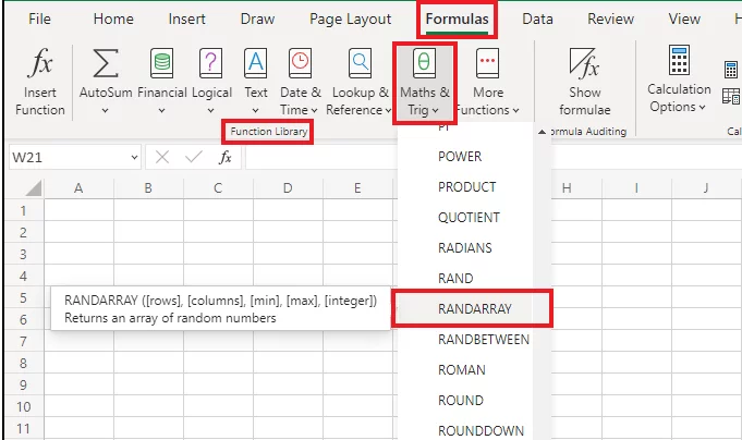
You can access it from your Functions Library as follows.

Formulas > Functions Library > Math & Trigonometry > RANDARRAY

 

 

Why would anyone want to use it?

Fields like science, arts, cryptography, statistics, computer simulations, and prototyping extensively use random numbers. Random numbers are used for testing, experimentation, and sampling purposes at multiple levels.

Also, as the human brain can never be utterly rational at picking truly random numbers, Excel can be of great help for random number generation.

 

RANDARRAY Use Cases

As a successor to the contemporary random number generating functions, the RANDARRAY function can be used for multiple causes. Find some of them listed below.

1. One of the best uses of the RANDARRAY function is to pick out a truly random sample from a finite population. This can be for verification or grouping purposes.
2. RANDARRY function can be used to introduce irregularity and unpredictability in a given set of numbers to be used for auditing purposes.
3. Many statisticians, researchers, and scientists use random series for hypothesis and prototyping.

Learn about other useful new dynamic array functions of Microsoft 365 such as the SEQUENCE function and SORTBY function.

Using RANDARRAY To Return An Array Of Random Numbers – Simple Example

Through the example below, let us quickly learn the basic application of the RANDARRAY function that generates random numbers.

Going very basic, let us generate a range of random numbers between 20 to 70 which is 4 rows tall and 5 columns wide.

Step 1:

To have a series of random numbers plotted as said above, the first step is to ensure you have enough empty cells to plot the same.

As the random number range is going to spill across 4 rows and 5 columns, you must have the next four rows and the next five columns vacant. The count starts from the first cell of the series where the formula is entered.

Step 2:

Activate the designated cell and compose the RANDARRAY formula as below.

= RANDARRAY (4, 5, 20, 70, 1)

What have we done?

• • The first argument of Rows is set to 4 as we want a 4-rows tall range of random numbers.
  • The second argument of Columns is set to 5 as we want a 5-columns wide range of random numbers.
  • As we want our random numbers to range between 20 and 70, the minimum value is set to 20 and the maximum value is set to 70.
  • We only want random integers to the range, so the fourth argument is set as 1 i.e. TRUE. To populate decimals in the range, it can be set to 0 i.e. FALSE, or can be omitted.

Step 3:

After the formula is all composed, hit ‘Enter’ to yield results as follows.

 

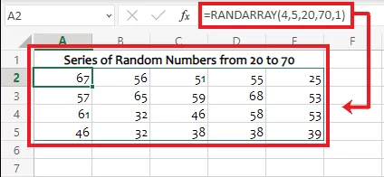
According to the arguments specified, Excel has generated a series of random numbers starting from 20 up to 70 consisting of whole numbers only.

More Examples

The foundational example stipulated above must have helped you learn how you can generate a simple series of random numbers using the RANDARRAY function in Excel.

It’s time we now progress towards learning how the RANDARRAY function can be used for advanced purposes.

1. Generating Random Dates using RANDARRAY

Is the RANDARRAY function only good to generate random numbers? Obviously not. You can use it for various purposes like generating dates.

The image below represents two dates that mark the beginning and end of the Spring festival.

 

 

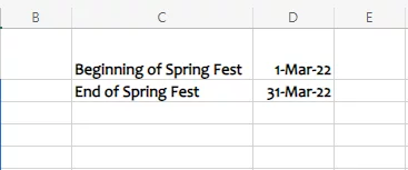
If you want to visit the Spring Fest for at 10 days on a random basis, how can you do that?

Step 1:                      

Clear out the spill range and compose the RANDARRAY function as follows.

= RANDARRAY (10, 1, D1, D1, 1)

• • • We want to find out the next 10 random dates. The number of rows is therefore, set to 10, whereas the number of columns is set to 1 through the first and the second argument respectively.
    • The minimum number from where we want the range to start is set as the beginning date and the maximum number is set as the ending date. This is because we want to find 10 random dates between these two dates.
    • The fourth argument is set to 1. It can also be omitted.

Step 2:

Press Enter to find the 10 random dates to visit the Spring fest.

 

 

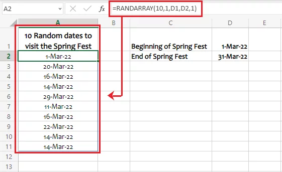
Excel has generated 10 random dates between the starting and ending dates supplied.

Pro Tip:

Do your results look more like this?

 

 

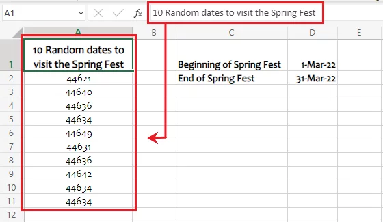
This is because you haven’t formatted the cells right. Select the underlying cells and format them as dates by going to Home > Number > Number formats > Short date.

Excel would turn the above serial numbers into dates.

 

2. Generating workdays using the RANDARRAY function

Continuing the same example as above, what if the festival is only held on weekdays and not on Saturdays and Sundays? Not to worry, the RANDARRAY function can also generate a series of random workdays.

To find only workdays from the above example, nest the RANDARRAY function into the WORKDAY function.

Step 1:

Compose the RANDARRAY function as follows.

= RANDARRAY (10, 1, D1, D2, 1)

This will generate a series of random dates between the first and last dates of the Spring Fest.

Step 2:

Nest the above RANDARRAY function into the WORKDAY function to only generate workdays and not weekends.

= WORKDAY (RANDARRAY (10, 1, D1, D2, 1), 1)

Step 3:

Press Enter to see the results as follows.

 

 

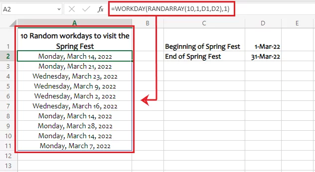
Pro Tip: Format the date type to include the day and see the workdays generated by Excel.

 

3. Picking out a sample through the RANDARRAY function

The first thought our brains hit at when we hear of random numbers is sampling. But how can we fetch out a sample in Excel from a given series of random numbers? Learn below.

The data below represents the unique number of different purchase invoices.

 

 

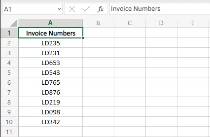
How can you draw a sample of 5 invoices from the given set using RANDARRAY?

Step 1:

Set up the RANDARRAY function as follows.

=RANDARRAY (5,1,1,9,1)

• • • The above function specifies 5 and 1 against the rows and column argument, respectively. This is the number of sample invoices to be drawn i.e. 5.
    • 1 and 9 as the third and fourth arguments specify the minimum and maximum values. We need RANDARRAY to pick out any 9 random numbers. These 9 numbers will be used against the INDEX function to pick out the invoice numbers at each respective row number.
    • We have used 9 as the maximum value as the total population consists of 9 invoices only.
    • The whole_number argument is set to 1 as the INDEX function needs whole numbers as row references to pick out the invoice value against the same.

Step 2:

The next step is to nest the RANDARRAY function into the INDEX function. Do it as follows:

= INDEX(A2:A10, RANDARRAY (5,1,1,9,1))

The INDEX function works on the premise that we specify a range and a row number. The Index function returns the value from that range against that row number.

In the above formula, we have used the INDEX function to return the row value (Invoice number) against each of the random numbers picked up by the RANDARRAY function.

Step 3:

Press ‘Enter’ to draw a set of 5 sample invoices as shown below.

 

 

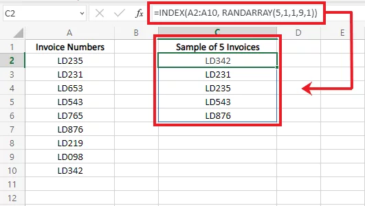
That is how you can draw a sample from any population making the above formula work for different datasets.

To avoid duplication of data in the random numbers, the RANDARRAY function may be nested into the UNIQUE function.

RANDARRAY Troubleshooting

Below are some common problems encountered by users while using the RANDARRAY function. Be mindful of them to have a seamless experience generating random numbers using the RANDARRAY function.

1. #NAME! Error

Excel would usually pose the name error for one of the following reasons.

• • You are using an outdated version of Excel that doesn’t support the RANDARRAY dynamic array tool.
  • Or you have spelled RANDARRAY incorrectly.

Take a quick look into the possibility of both the above reasons when faced with the #NAME! error in Excel.

2. Automatic Regeneration

Alike RAND and RANDBETWEEN, the RANDARRAY function is a volatile one. This means, as soon as the worksheet is recalculated, the RANDARRAY function would regenerate a new list of random numbers.

However, if you want to stick to a particular series of random numbers without it changing, again and again, you may copy, and special paste them as simple values.

3. Inappropriate Minimum and Maximum value arguments

The third and fourth arguments of the RANDARRAY function that specify the minimum and maximum values of the random series have to be logical. If you set the minimum and the maximum value as 5 and 1, respectively, Excel would only give back the #VALUE! Error.

The minimum value must be smaller than the maximum value.

4. No arguments specified

As discussed above, all four arguments to the RANDARRAY function are optional. Does that mean you can omit them all and operate the RANDARRAY function blank?

Yes. But what would the results look like?

 

 

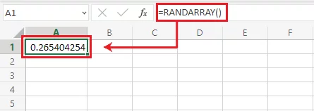
If all the arguments are omitted, the RANDARRAY function generates a single random number by setting the minimum and maximum values to 0 and 1, respectively.

 

Conclusion:

It’s time we advance the simple random number generating functions by shifting to the RANDARRAY function. It is not only easy and versatile, but has many additional features to offer.

Need an overview of everything Arrays can do in Excel? Check out our guide to Excel array formulas here.