
How To Take Advantage Of Logical Functions In Excel!
Contents
Anyone that studied maths knows how powerful logical functions can be.
And if it wasn’t, then this guide is all you need to become proficient in the logical functions in Excel.
The details are given below, so let’s dive right into the topic.
What are Logical Functions in Excel?
Even if you’re not familiar with what these functions entail, you must have heard their name before.
Logical functions are some of the most important and common functions in Excel.
They work as a decision-making tool for dealing with information.
Logical functions also allow you to use conditional formatting in between the formulas.
Excel Logical functions test a condition to check if it is TRUE or FALSE.
It then allows to perform further operations on the data depending on the logical test result.
You select a cell, enter values and apply a logical function. Now you can calculate the data using the formula or test the situation against a fixed logical value.
Excel offers more than ten logical functions, but the most basic ones include AND, OR, NOT, XOR and IF.
These functions are the most used for performing logical operations, while other functions include SWITCH, TRUE, FALSE, IFERROR, IFN/A, and IFS functions.
The first four functions are pretty easy to use, and they come in handy when you want to test multiple conditions or perform a bunch of evaluations. If the logical value is correct, it returns TRUE and false if incorrect.
AND Function
The AND function is one of the most commonly used functions in Excel.
It comes into use when you want to compare more than two values.
The AND function returns TRUE when all the conditions are met and FALSE even if a single condition is wrong.
Also, it is used in combination with other functions and is a fine alternative to the IF NESTED function.
Syntax
=AND(logical1, logical2,..)
Where logical is the expression or condition that you need to assess. This expression can be anything from a cell reference to the text, numbers, etc. The first expression is compulsory, while others are optional for the formula.
Formula Example
=AND(A2>10, B2>5)
Here’s how it works
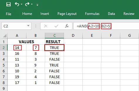
The AND function returned TRUE after checking if both the cells fulfilled the condition. If any one of the cell values had not met the condition, the AND function would have returned FALSE.
OR Function
Similar to the AND function, the OR function is also used to differentiate or compare two cell values. The primary difference is that, unlike AND, the OR function returns TRUE even if one cell value does not meet the required condition.
It returns FALSE only when both the conditions are not met. OR function is widely used in Excel for numerous purposes, and it is often used in combination with other functions like NESTED IF, etc.
Syntax
=OR(logical1, logical2)
Where logical1 is the first condition to be evaluated with the same requirements as the AND function.
Formula Example
=OR(A1>10, B1>5)
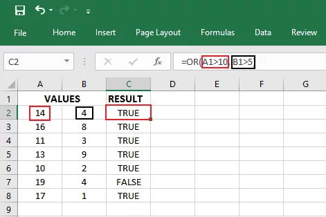
As evident, the formula used in this example is the same as AND function, and the only difference is that the values in cell B2 were changed. Now, cell B2 does not meet the condition, but the OR function returns a TRUE value, as explained above.
It would have returned FALSE if neither of the conditions were met.
NOT Function
NOT function performs the easiest of operations. It simply reverses the logical result, meaning if the answer of two conditions evaluates to TRUE, by applying the NOT function, the return value will now be FALSE and vice versa. It can be combined with other functions like OR, AND, etc.
It’s fair for you to question why anyone would want to do something so bizarre. The answer is, often you want to see where a condition isn’t being fulfilled rather than where it is being fulfilled. And NOT function is your best option in such a case.
Syntax
=NOT(logical)
The ‘logical’ in NOT function is the argument to be negated.
Formula Example
=NOT(5+5=10)
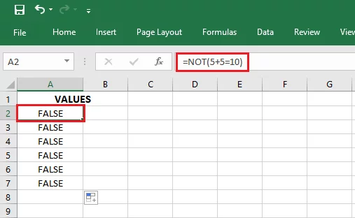
Here the NOT function returned FALSE when the condition evaluated to TRUE, i.e., it reversed the value.
XOR Function
XOR function stands for Exclusive OR function, and it operates similar to the OR function with a slight difference only.
The XOR function returns TRUE when only one argument is TRUE. If both the arguments are TRUE or both the arguments are FALSE, it will return FALSE.
Syntax
=XOR(logical1, logical2)
Where logical is the condition to be evaluated. A single formula allows 254 values to be tested with the XOR function.
Formula Example
=XOR(A2>8, B2=6)
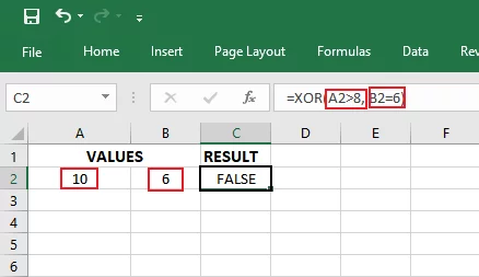
In this example, the return value is FALSE because both the conditions are met.
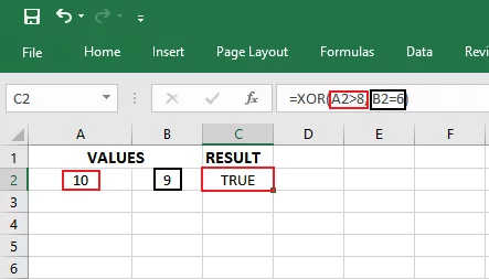
The return value is TRUE in this example since the condition in A2 is met, but the condition in B2 is not fulfilled. The same would happen if both the conditions were not to be met.
IF Function
The IF function is undoubtedly one of the most used functions in Excel and for various purposes. The IF function checks a condition, whether it is TRUE or FALSE. Based on the result, it returns a specific value when TRUE and another when FALSE.
IF function is mostly used in combination with other functions and has several other types, including IFS, IFERROR, etc. Using the IF function is easy if you know how the following formula works.
Syntax
=IF(logical_test, value_if_true, [value_if_false]
Where logical_test (mandatory) is the condition to be evaluated, Value_if_true is the argument (required) that is to be returned if the result is TRUE. Value_if_false is the argument (optional) that is to be returned if the result is FALSE.
Formula Example
=IF(A1<=10, ‘Yes’, ‘No’)
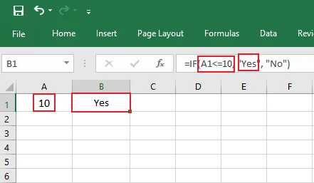
In this example, the IF function returned Yes because the cell value of A1 met the condition required. Otherwise the IF function would have returned No.
COUNTIF Function of Excel is an advanced for of the IF Function. It allows users to count the number of values in a data set only if they meet a specific criterion.
IFS Function
The IFS function tests one or more expressions and returns a specified value on TRUE result. It checks the first condition; if TRUE, it utilizes that. If FALSE, it moves on to the second condition and so on in the subsequent order.
The IFS function is better at running tests and checking conditions than the regular IF function. IFS function allows you to add up to 127 logical statements in a single formula.
Syntax
=IFS(logical_test1, value_if_true1, [logical_test2], [value_if_true2], …)
Where logical_test1 is the first condition to be tested. If TRUE, the function does not evaluate any further and stops right there. If FALSE, the function then tests the second condition (if any) and utilizes that value. Value_if_true1 is the value to be returned if the first condition evaluates to TRUE.
Formula Example
=IFS(A2>90,”A+”,A2>80,”A”,A2>70,”B”,A2>60,”C”,A2>50,”D”,A2>40,”E”)
In this example, the return value of the IFS function is YES because the condition applied was TRUE. If the condition had been FALSE, the IFS function would have returned the NO value.
The IFS Function of Excel is commonly used in pair with Forecast sheets in Excel. Learn all about forecasting in Excel here.
IFERROR Function
As evident from the name, the IFERROR function is used to deal with errors in a function. It locates the error and returns the specified value if an error occurs. Otherwise, the IFERROR function returns the result of the formula entered.
Syntax
=IFERROR(value, value_if_error)
Where value is the argument (required) that is to be evaluated for any error. The value_if_error is the argument to be returned when an error occurs.
Formula Example
=IFERROR(A2/B2, “Error in calculation”)
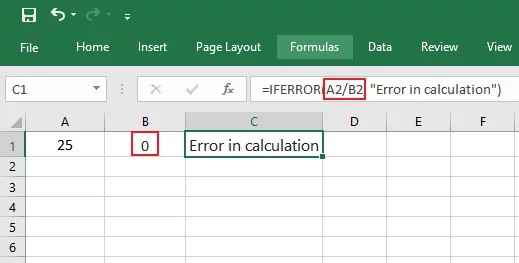
The IFERROR function returned an Error in the calculation because division by zero gives an error, so it displayed the value-if-error.
IFNA Function
As evident from the name, the IFNA function is used to locate and remove the NA error in a formula. When the NA error is encountered, it returns a default value stored in the formula. Otherwise, it returns the result of the formula.
It is only available in Excel version 2013 and above.
Syntax
=IFNA(value, value-if-NA)
Where value is the expression or cell reference to be checked for the NA error, and the value if NA is the result to be returned in case an NA error occurs.
Formula Example
=IFNA(A1/B1,0)
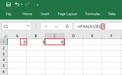
The formula returned zero because the first cell value has zero as a digit.
TRUE Function
The TRUE function returns the value TRUE based on an argument or expression. It is built-in in Excel and acts like a worksheet function. The following formula is used for the TRUE function.
Syntax
=TRUE()
Where TRUE is the value returned as an answer to the expression.
Formula Example
=IF(A1=22,TRUE())
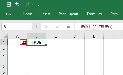
In this example, the formula returned TRUE since the given condition was met.
FALSE Function
The FALSE function works like the inverse of the TRUE function; depending upon the condition entered, it returns a FALSE value. It is also a built-in function and is used as an Excel Worksheet function.
Syntax
=FALSE()
Where false is the value to be returned upon evaluation of the condition or expression.
Formula Example
=IF(A1>47, FALSE()
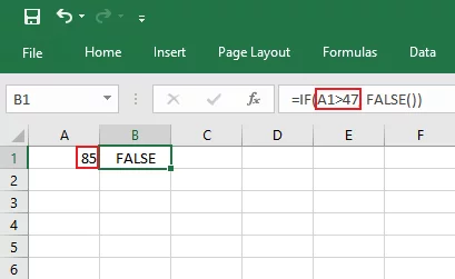
In this example, the formula returned FALSE as the given condition was TRUE.
SWITCH Function
The SWITCH function is used to test a single value against multiple other values. As a result, it returns the value that matches the first corresponding value. When no value matches the first one, the SWITCH function returns a default value that the user can set.
Syntax
=SWITCH (exp, value1/result1, [value2/result2], …, [default])
Where expression is the value (mandatory) that is to be matched against. Value 1/result1 is the first value to be matched along with the resultant value and is required. Value2/result2 is optional.
Formula Example
=SWITCH(A2,0/”Poor”,5/”OK”,10/”Good”,”?”)
In this example, the SWITCH function returns remarks corresponding to their entries. You can even use conditional formatting in the SWITCH function to know which value is greater or smaller than the set criterion.
Logical Functions – Use Cases
Given the scope and wide usage in Excel, Logical Functions can be used for almost any purpose. And these functions can be used by anyone, ranging from beginners on Excel to corporate firms, anyone. Let’s see some of the uses a logical function has to offer as below:
Use Case 1:
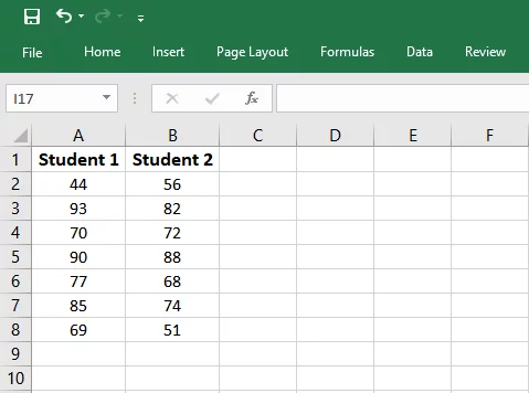
Say, you need to compare the marks of two students and find out where one has scored less than the other and vice versa. Here’s how you can set up the main logical function AND function for this purpose.
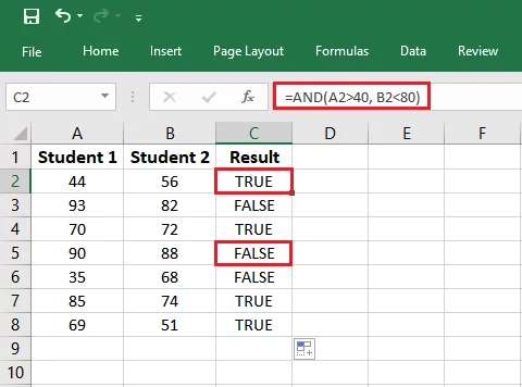
Apply the AND function as follows:
=AND(A2>40, B2<80)
Where A2 are the marks of the first student and B2 are marks of the second. If both the conditions are met, the AND function will return TRUE and FALSE if any one of the two is FALSE.
At any point where the AND logical function observes marks less than 40 or greater than 80, it returns FALSE for that value. Here’s what it looks like:
You may also highlight specific values based on a defined parameter (for e.g. marks). Learn all about conditional formatting in Excel here.
Use Case 2:
While forming budgets or sorting monthly expenses at home, you may realize you blew some extra funds. To identify where you went off-limit, here’s how you can use the IF function.
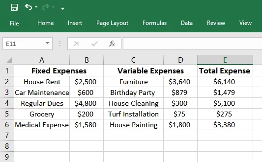
Apply the IF function as follows:
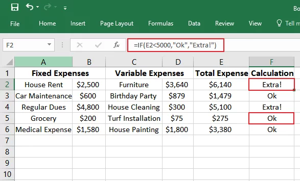
=IF(E2<5000,”Ok”,”Extra!”)
In this example of the IF function, cells with ‘Ok’ will show that the expenses are under $5,000, whereas the ones with ‘Extra!’ inform where the expenses exceed the set limit.
The result of the IF function is as follows:
Logical Functions – Simple Example
Using logical functions for daily life problems is pretty simple once you become well-equipped with their formulas and usage of arguments. You can use them to find the best of two values, for electing the correct values, adding remarks, and a lot more. Let’s see an example of the working of a logical function as below:
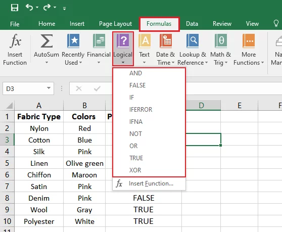
In the screenshot below, the fabric type and colors exemplify the source data to be dealt with.
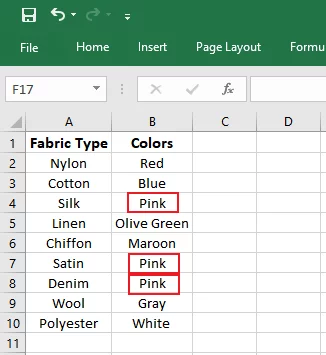
Apply the formula as follows:
=NOT(B2=”Pink”)
Of all the colors, we do not want the fabrics in the color pink. So to pin out the said colors from this list, we bring the NOT function to our help.
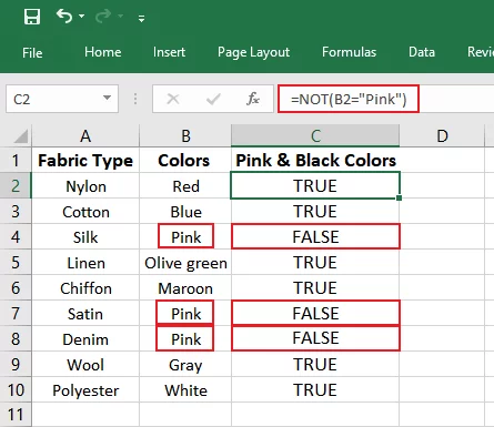
The NOT function returned TRUE for cells containing colors other than Pink and False for the cell values containing Pink.
Additionally, you can find the logical functions in Excel by following the given course.
Formulas > Function Library > Logical Functions
Want to learn more about Excels most powerful features? Learn about the UNIQUE Function here.
Conclusion
Logical functions play a crucial role in our lives today, from solving daily life problems to businesses handling data, it works everywhere.
They offer an array of functions to choose from to perform different tasks.
And they are well-known because of the ease of use and steady results they provide.
Mastering logical functions can indefinitely help you in every field of life, and you can begin by practicing the above-given formula examples.
Mastering the fundamentals is key to not making mistakes – did you know 98% of people have seen an Excel error cost their employers’ money to fix?
For more fascinating facts, look at our Excel Research here.
Using logical functions, you can efficiently analyze your data in Excel. Click here to master data analysis in Excel.


- Facebook: https://www.facebook.com/profile.php?id=100066814899655
- X (Twitter): https://twitter.com/AcuityTraining
- LinkedIn: https://www.linkedin.com/company/acuity-training/