Excel Guide: Conditional Formatting [In 5 Minutes!]

 

Conditional Formatting formats a cell or group of cells based on your own conditions.

There are a lot of options, but they are all simple to implement with this guide!

On our Excel Courses, we teach a wide range of conditional formatting options, and they are simple to implement in your worksheets.

Simple Example – Conditional Formatting

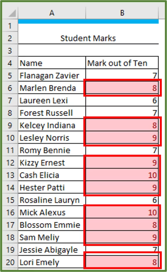
Our data set has student grades for a test.

We want to highlight everyone that scored above 10.

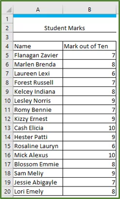
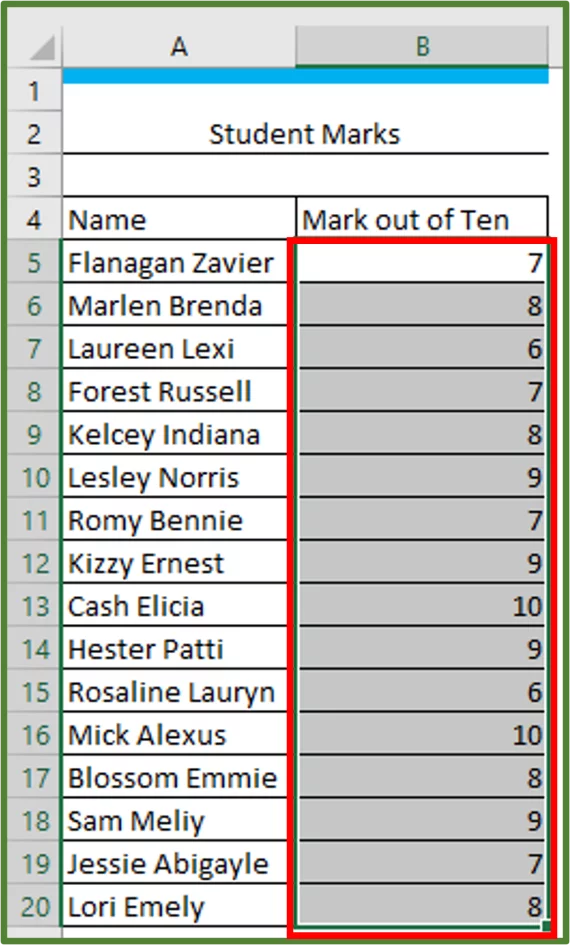
Select cells B5:B20.

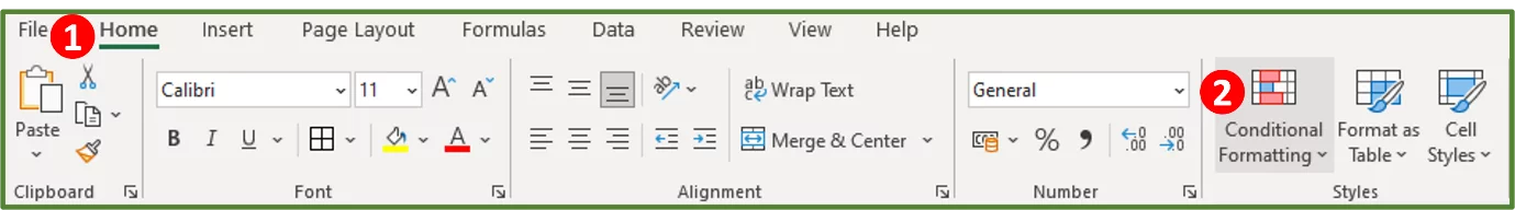
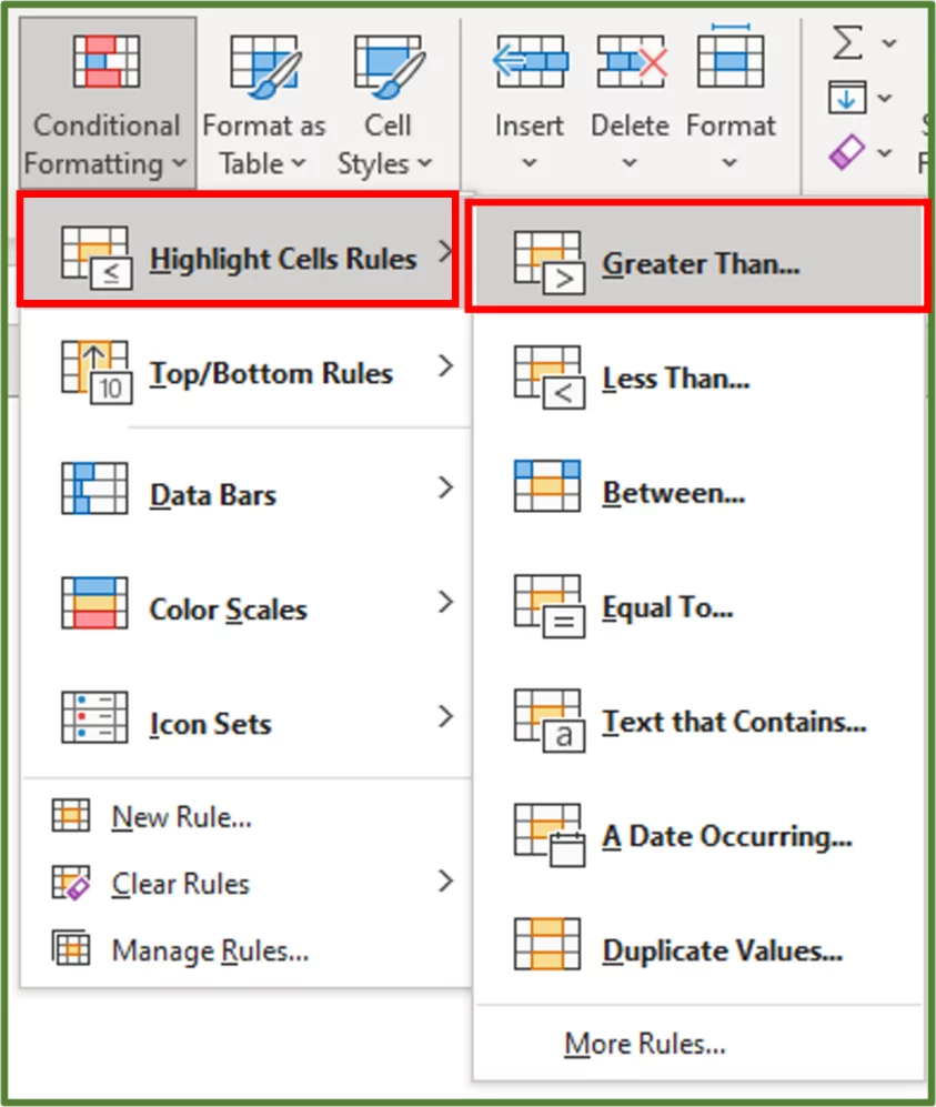
With cell range B5:B20 still selected, go to the Styles group on the Home Tab (Step 1 in the image) and select Conditional Formatting (Step 2 in the image).

Select Highlight Cells Rules and then Greater Than…

The Greater Than Window should appear.

Enter 7 in the textbox underneath the Format cells that are GREATER THAN: section and leave the format as Light Red Fill with Dark Red Text.

Click Ok.

All the cells that contain a value greater than 7 should now be highlighted with the Light Red Fill with Dark Red Text.

You can also use conditional formatting to make heat maps in Excel.

Using Custom Conditions

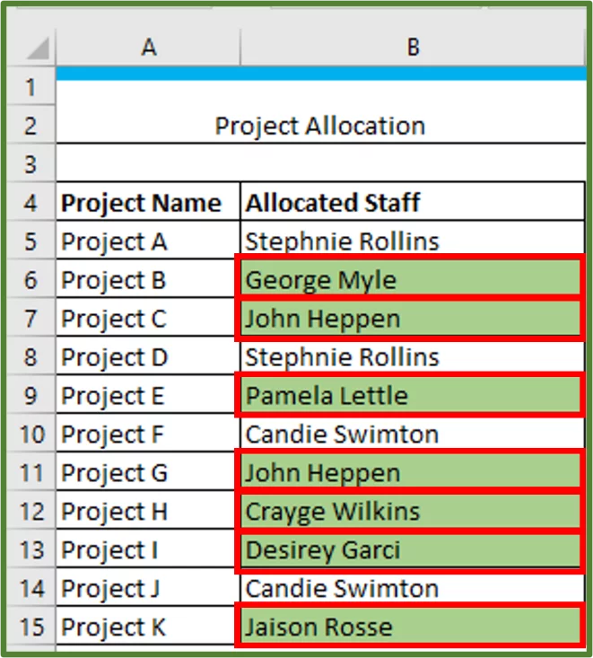
You can create your own formulas for custom conditions. In our example, we have a list of projects and the staff member responsible for the project recorded.

We want to see which staff members other than Stephnie Rollins and Candie Swimton are responsible for projects. So, we will need a custom condition.

Select the cell range B5:B15.

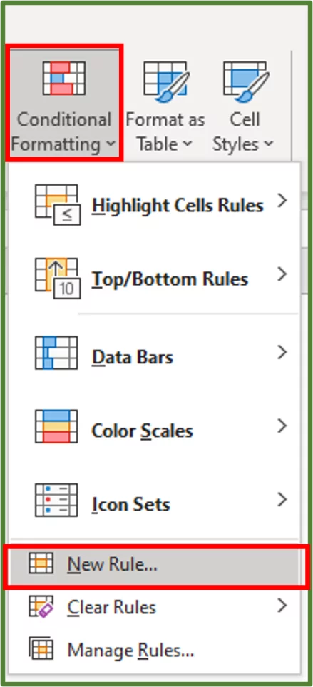
With this range selected, go to the Styles group on the Home Tab and select Conditional Formatting and choose New Rule…

The New Formatting Rule Dialog Box should appear.

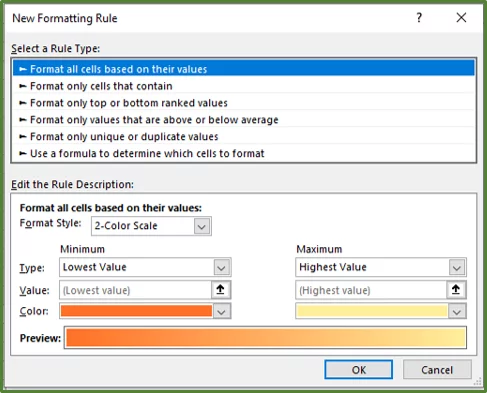
Select the Use a formula to determine which cells to format option.

This lets you use Functions and Formulas to write your own rules!

 

Excel will start by looking at the value in cell B5 and then going down the rows in the selected range and only format those names that are not Stephnie Rollins or Candie Swimton.

Click on the Format… button, and you can choose any format that you’d like, but in this case, we are going to use a light green fill.

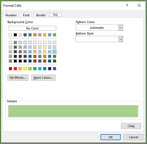
Click Ok. You should now see a preview of what the formatting will look like.

Click Ok again. The staff other than Stephnie Rollins and Candie Swimton are highlighted.

Clear Conditional Formatting from Cells

If you would like to clear the conditional formatting from your cells or worksheet. You can do so in the following way.

Select the cell range containing the conditional formatting, which in this case is range B5:B16.

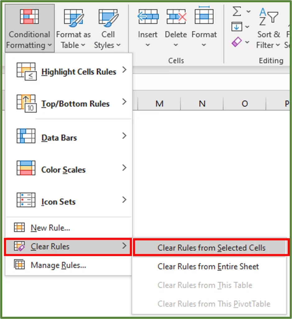
With this range selected, go to the Styles group on the Home Tab and select Conditional Formatting.

Choose Clear Rules and then Clear Rules from Selected Cells.

The conditional formatting should now be cleared from the selected cells.

Conclusion

Excel’s conditional formatting options are powerful and allow you to format data according to simple criteria and to use your own formulas for more advanced criteria.

You will often see conditional formatting applied in advanced dashboards and reports.

Casual Excel users and professional Excel users can make use of the conditional formatting options that Excel provides, and it’s available on Excel for Web as well for easy collaboration with colleagues.

Another case where conditional formatting can be used is when looking for outliers in a dataset!

Special thank you to Taryn Nefdt for collaborating on this article.