Finding Outliers In Excel: A Detailed Guide

Microsoft Excel is an incredibly powerful data analysis tool that empowers users to store, analyse, and visualise data to derive valuable insights out of it.

With so many basic and advanced level data analysis tools, Excel provides you with almost everything that you need to cater to volumes of information. An important part of data analysis in Excel is to identify any anomalies within a data set that may defy its statistical norms. We call these outliers.

To introduce the topic briefly, outliers are data points that stray from the core of a data distribution. If not handled appropriately, they can jeopardise the validity of your statistical analysis. How, why, and what can help it? Find answers to all these questions in the guide below.

If you would like to master the different tools within Excel, from beginner to advanced, with the help of an experienced trainer, our Excel courses might be ideal for you. Check out the different training options available on our website.

What Are Outliers?

Generally, we can expect the values in a data set to be in fair symmetry from their median (centre point). But if some values of that data set are way beyond the range of that data, we call them outliers.

Simply put, these are abnormally high or low values within a data set that may occur because of measurement errors, data entry mistakes, or genuinely unusual phenomena.

Don’t take them lightly – they can skew your data really bad. How? Let me show you that on a very basic level by considering the following data set.

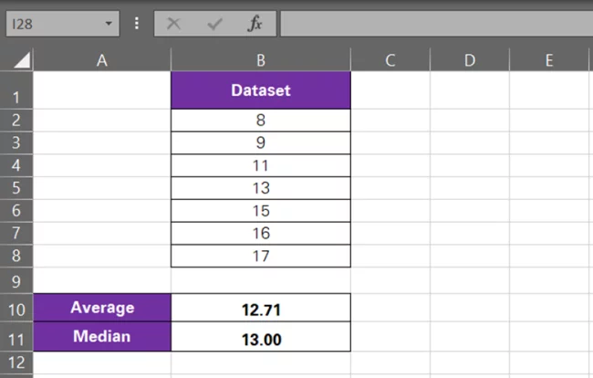
8, 9, 11, 13, 15, 16, 17

The lowest value of the data set is 8, and the biggest value is 17. Arranging the values in ascending order, we understand that there is a gap of 1–2 between each value of the data set.

Very clearly, the median of this data set is 13. And the average for the same turns out to be 12.71, ~ 13.

Now, if we tweak the data set a little to include some other numbers, this is how the average changes.

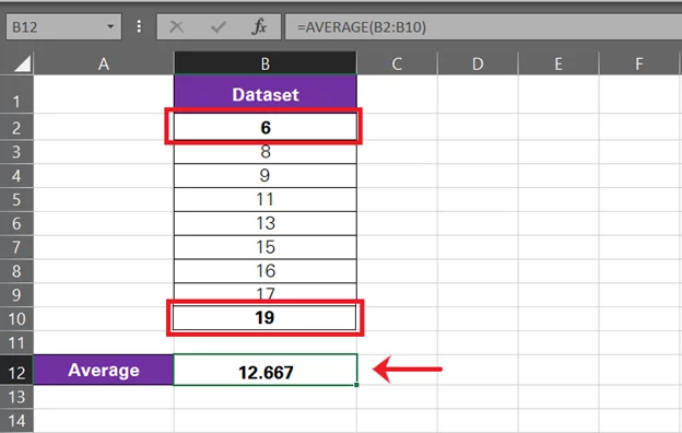
The average for this data set sees a slight change from 12.71 to 12.67 (barely noticeable). This is because the new numbers added were not oblivious to the existing data set. They were well in range.

But let’s tweak this data set as follows:

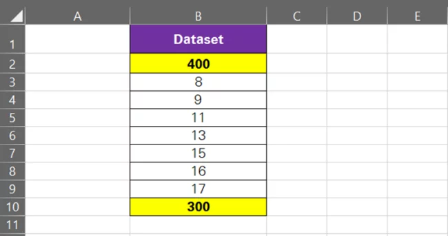
The numbers added this time are 300 and 400.

Both numbers are extreme data points and do not blend in very well with the existing data set. Here’s how the average of the data set moves to capture the effect of these numbers.

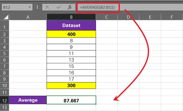
The average jumps from 12.71 to 87.667 – quite some jump. Most of the numbers in the data set are around 8 to 18, but only two out-of-the-range numbers make things odd.

That’s how outliers skew the inferences to be drawn from a data set.

Clearly, 300 and 400 are outliers in this data set.

Why Is It Important To Detect Outliers In Excel?

We’ve seen outliers from a statistical perspective: what they are, and how they can distort data. But how can outliers result in anomalies and incorrect decision-making in our daily lives?

Let me show you a practical example here.

Assume you live in Street 15 of XYZ Block, and your office is situated nine miles from your home in JKL Block. Cool. What’s the average Uber fare from your home to your office?

To reach that number, we have collected stats from a week of Uber travelling between both locations.

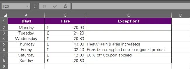
P.S.: The fare usually stays in the ambit of £20–£21. However, on a few days, we see some exceptional fares due to heavy rains, peak factors, and sometimes coupons.

Now, what’s the average fare for a nine-mile ride?

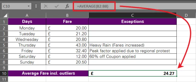
The average turns out to be £24.27, which is not the true average fare. It should be somewhere around £20. The reason for the average being skewed is the inclusion of exceptional fares in the stats (what we call outliers).

An average of £24.27 means you’d have to pay around £24 every day for travelling from your office to home. Whereas, actually, unless there’s an exceptional situation, the fare for this distance is no more than £21. Taking £24 as the average fare would lead to uninformed decision-making and inaccurate budgeting as it fails to account for the outliers in the fare stats.

That’s how outliers can impair your decision-making in practical life. To make sure you’re reading your data correctly and arriving at the right analysis, make sure your data is checked for any outliers.

Let’s leave out the outliers from these fares and recalculate the average fare as below.

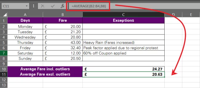
This time the average fare comes off truer – £20.63.

Practically speaking, we have come down to the answer to ‘Why is it important to detect outliers from a data set?’ Because, if you do not detect and handle outliers within a given data set before you process it, there’s a high chance you’d pull out inappropriate conclusions.

Some other potential consequences of not addressing the outliers of your data set include:

1. Using biased statistical analyses that lead to unreliable and inaccurate results – means, medians, standard deviations, and other stats.
2. Generalizing the findings of a data set for a broader population becomes impossible.
3. Impeding the value driven by predictive modelling like regression analysis, cash flow forecasts, etc.
4. Missing important findings if outliers are not investigated. Outliers often represent areas that require assessment and improvement. For example, if you’re collecting the stats on the spread of XYZ disease in every region of the world, and some regions show abnormal numbers as compared to the rest, they might warrant special attention. Outliers help identify such anomalies for further investigation.
5. Failing to identify outliers casts doubt on the reliability of the data, leaving it less representative of the underlying population.

Methods To Calculate Outliers In Excel

Guess we have had quite some pep talk about what outliers are, what they do, and why it is necessary to pick them out. It’s now time we see how to find outliers.

There are several ways you can detect outliers in Excel, but first, we need to calculate them.

Calculating outliers for a given data set is something more subjective, and you can choose a suitable criterion for identifying them yourself. Two methods that are commonly used to calculate outliers are:

1.    The Interquartile Range

The word quartile is a derivation of the word ‘quarter’, which means 1/4.

Just like a clock, the quartile formula divides a given data set into four parts. The median of each of these parts is what we call Quartile 1, Quartile 2, and Quartile 3.

The Interquartile range is the measure of the middle-half spread of the data that is not affected by outliers. It comes out as the difference between the 3rd and the 1st Quartile:

= Quartile 3 – Quartile 1

The IQR method is a very robust measure of averaging out data. With this method, you calculate a lower and upper limit for the values in your data set. Any value that goes beyond these limits makes a potential candidate for outliers. Simple enough.

How about playing around with an example to see how this works?

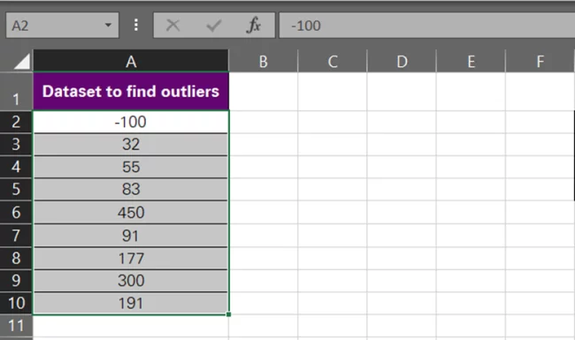
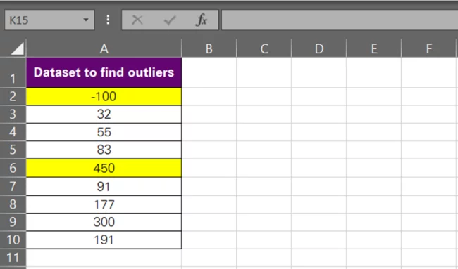
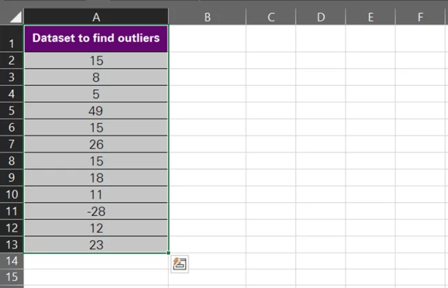
Calculating outliers through the IQR rule in Excel is all about putting a few formulas and functions in order. For example, here we have a data set.

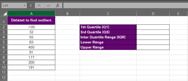
To find the outlier threshold for this data set using the IQR rule, follow the steps below:

1. 1. Find the first quartile for your data set by writing down the quartile function as follows:

= Quartile (A2:A10, 1)

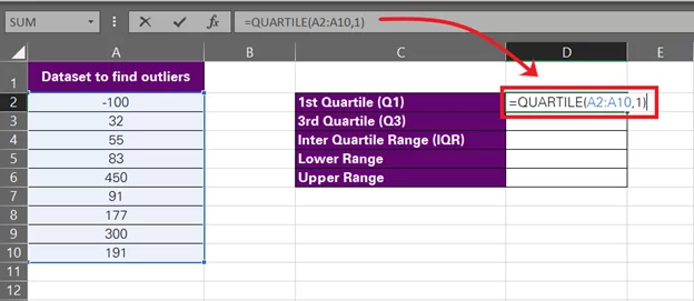
We have specified the array that contains the data set, i.e. A2:A10. Since we want to find Q1, we have set the quart argument to 1.

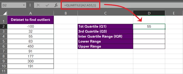
And here we have the first quartile.

1. 2. Next, find the 3rd Quartile (Q3) similarly.

= Quartile (A2:A10, 3)

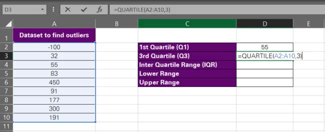
Everything remains the same except for the quart argument that is now set to 3, as we want to find the 3rd quartile (Q3).

1. 3. Hit ‘Enter’ for the following results.

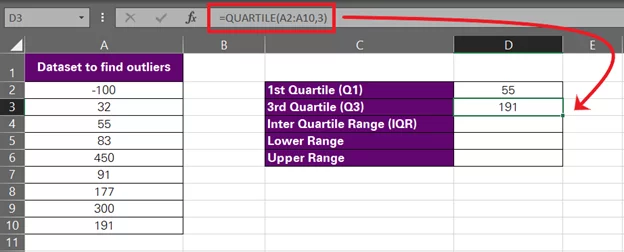
Finding quartiles with Excel is easy.

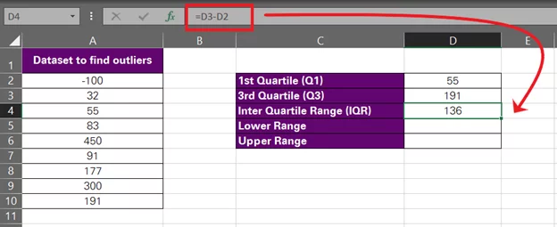
1. 4. Find the interquartile range for this data set by finding the difference between the third and the first quartile.

= Q3 – Q1

As we have the values for Q3 and Q1 populated in cells D3 and D2, respectively, our formula would change to:

= D3 – D2

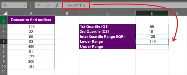
1. 5. To find the lower outlier (abnormally small values for this data set), we will use the following formula:

= Q1 – (IQR*1.5)

Using relative references for the cells that contain these values, here is how it looks:

= D2 – (D4*1.5)

1. 6. Next, find the upper outlier limit through the following formula:

= Q3 + (IQR*1.5)

Using relative references for the cells that contain these values, here is how it looks:

= D3 + (D4*1.5)

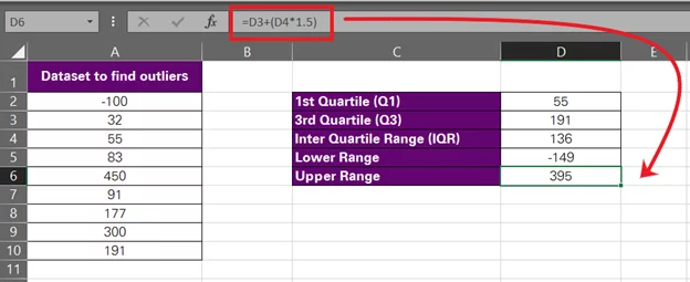
So, now we have the lower and upper outlier thresholds as -149 and 395. Per the IQR rule, any data points in our data set that fall outside the range of -149 to 395 will be outliers.

Pro Tip!

The IQR rule of finding outliers says that any number of a data set that is smaller than the ‘difference of its first quartile and 1.5 times the IQR’ is an outlier on the lower end of the range.

Similarly, any number of a data set that is greater than the ‘sum of its third quartile and 1.5 times the IQR’ is an outlier on the higher end of the range.

The number 1.5 is arbitrary. You can replace it with the desired number of IQR (2, or 3, or anything). We are going with 1.5, as it is the most used and accepted, in the world of stats at least.

2.    Standard Deviation

Another less commonly used method for finding outliers is the standard deviation method. Let’s continue with the same data set as above.

Here’s how we will find the outlier threshold for this data set using the standard deviation method:

1. 1. The first thing we’d do is calculate the average of the given data set. Let’s not bother much – we will put the AVERAGE function into action.

= AVERAGE (A2:10)

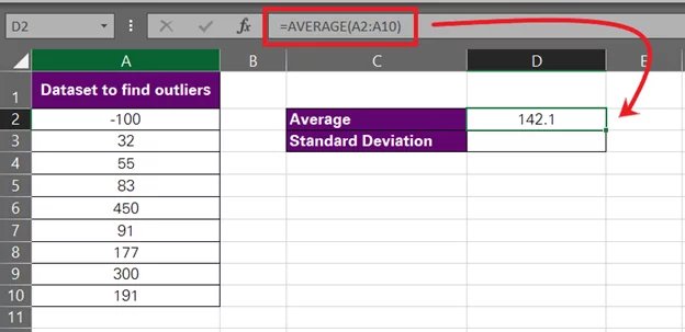
That’s around 142.1. Cool.

1. 2. Calculate the standard deviation for this data set using the STDEV.P function as follows:

= STDEV.P (A2:10)

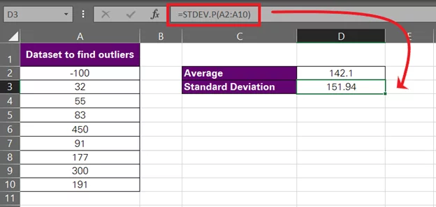
This comes out to be 151.94.

P.S.: Standard Deviation is the statistical measure of the degree of variation you can expect in a data set. It defines to what extent you can expect the individual values of a data set to differ from the central point.  

1. 3. Determine your criterion for defining outliers. Typically, any data point that is 1.5 times higher than the standard deviation of the data set is an outlier. However, you can set this to a different number, say 2, in which case a data point would be an outlier if it’s two standard deviations away from the average.

We are setting it to 1.5 for the moment.

1. 4. Calculate the upper and lower limits for outliers by using the following formula:

Lower Limit = Average – (Standard Deviation*1.5)

Upper Limit = Average + (Standard Deviation*1.5)

Replacing the values of this formula with the relative references from our example, here’s what we get:

Lower Limit: D2 – (D3*1.5)

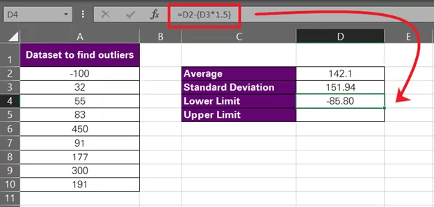
Upper Limit: D3 + (D3*1.5)

There we have it, -85.8 to 370.02.

In terms of the standard deviation method, any value in this data set smaller than -85.8 would be an outlier on the lower end of this data set. And any value exceeding 370.02 would be an outlier on the higher end of this data set.

Methods To Identify Outliers In Excel

We have seen two methods to calculate the outlier thresholds for any data set. It’s time we see how we can identify the outliers from our data sets.

Pro Tip!

You’d probably say, who needs a method for that? I will just scan through the data set.

Okay, you can do that for an exemplary data set like ours that goes no farther than nine values. However, as the number of values in a data set continues to grow, the process gets arduous, and visual scanning won’t help.

Let’s make it smart with some automated methods.

1.    Conditional Formatting

One of the basic ideas that must have struck your mind would be to formulate some setting that automatically highlights cells that exceed the outlier threshold. You’re right – that’s what we call conditional formatting.

For all the methods to identify outliers, we are going to use the outlier range we calculated using the Standard deviation method, i.e., -85.8 to 370.02.

This means we need to scan our data set for any values smaller than -85.8 or larger than 370.02 – the outliers.

Now, to identify which values from this data set qualify as outliers, we need to put some conditional formatting rules in place.

1. 1. Select the range where conditional formatting is to be applied. For us, this is going to be A2:A10.

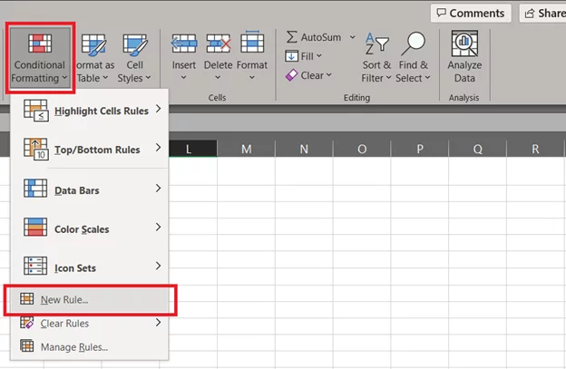
1. 2. Go to the Insert tab > Conditional Formatting button > New Rule.

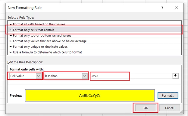
1. 3. Select the Rule ‘Format cells that contain’.
   4. Under ‘Edit the Rule Description’, make the following selections:

Cell Value | less than | -85.8

1. 5. Click Okay.
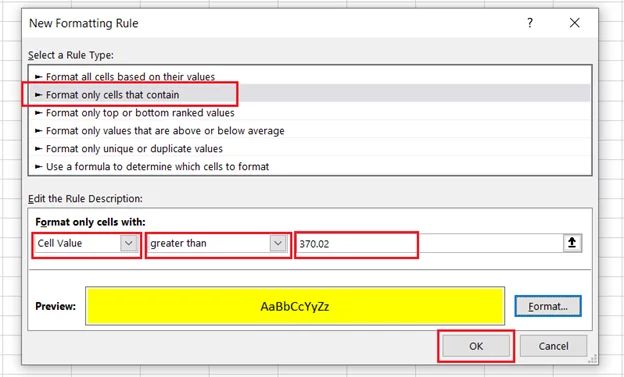
   6. Set up another rule by following the same steps as above for:

 Cell Value | greater than | 370.02.

1. 7. And Tada! All the outliers (values outside the range of -85.8 and 370.02) are highlighted.

Pro Tip!

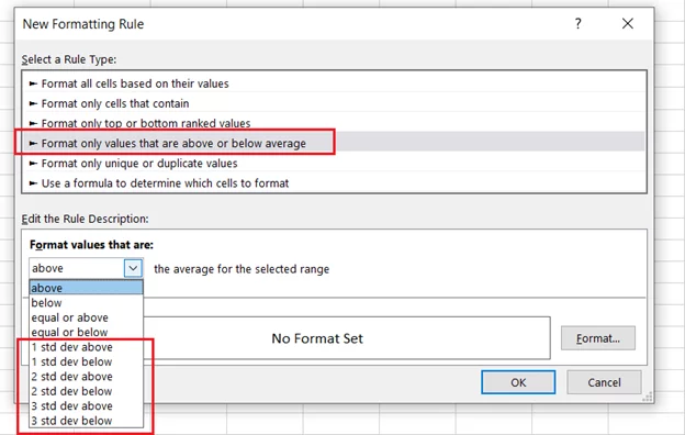
Conditional Formatting in Excel has an in-built rule to highlight values that are X standard deviations above or below the average of a data set.

Remember! This is the same formula that we used to calculate outliers under the standard deviation method.

Lower Limit = Average – (1.5 * Standard Deviation)

[Values that are 1.5 standard deviations below the average are outliers]

Upper Limit = Average + (1.5 * Standard Deviation)

[Values that are 1.5 standard deviations above the average are outliers]

The reason why we didn’t use this rule is that we have used 1.5 times the standard deviation in our formula, whereas Excel only allows 1, 2, or 3 times the standard deviation.

However, you can deploy this conditional formatting rule (as shown below) if you’ve set the number of standard deviations to 1,2 or 3.

2.    Using Formulas

Excel is all about formulas and functions, and what is it that you can’t achieve in Excel by tweaking different functions?

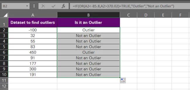
Want to detect outliers using formulas? We are going to nest the OR function into the IF function to detect if a given value is an outlier or not. Same data set and same outliers (-85.8 and 370.02).

Let’s go.

1. 1. Insert a new column next to the data set or wherever you want to have the results for each value populated.
   2. Begin writing the OR function.

= OR (A2 < -85,8, A2 > 370.02)

The above function translates to the question, ‘Is the cell value in A2 smaller than -85.8 or greater than 370.02?’

The value in A2 is -100, so the answer to this function would be true (first logical test true).

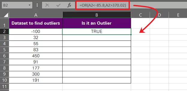
Note that the OR function is a logical function that returns the result ‘TRUE’ if any of the specified logical tests are true. It only returns FALSE when all the given logical tests fail.

1. 3. This OR function will become our logical test for the IF function.

IF = [Logical test, value if true, value is false]

= IF (OR (A2 < -85,8, A2 > 370.02) = TRUE,

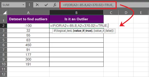
As the logical test of the IF function, Excel will check ‘If the OR function returns TRUE?’

If the OR function returns TRUE, the IF function will return the value_if_true. And if the OR function returns FALSE, the IF function will return the value_if_false.

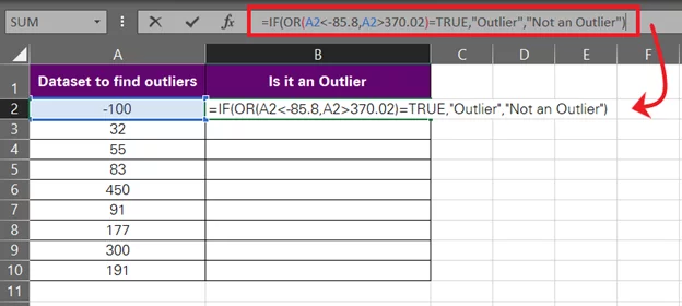
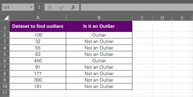
1. 4. Specify the value if true and the value if false for the IF function.

If the OR function returns TRUE, clearly the underlying value is an Outlier, and vice versa. We are accordingly setting the value_if_true as “Outlier” and the value_if_false as “Not an Outlier”.

= IF (OR (A2 < -85,8, A2 > 370.02) = TRUE, “Outlier”, “Not an Outlier”)

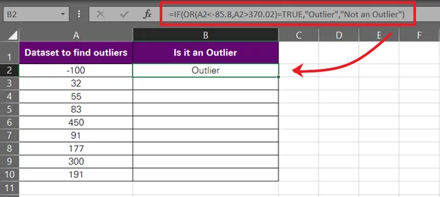
1. 5. Hit ‘Enter’, and there we have the result.

1. 6. Drag and drop the same to the whole list to make the formula work for the whole data set.

Easy? That’s how you can use multiple functions to build up a formula and have the outliers handpicked for you by Excel.

3.    Visual Inspection using Charts

This one has to be my favourite. Another way to identify outliers is to visualise your data set on a chart and track down the data values that exhibit an unusual behaviour. You can use several charts for this purpose.

We will look into the two most robust charts that will help you identify outliers from your data set at a glance.

Box and Whisker Chart

Here are the steps to be followed to identify outliers using a box and whisker chart:

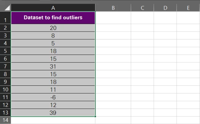
1. 1. Select the data set to be plotted on a chart.

 

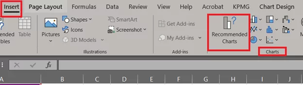
1. 2. Go to the Insert tab > Charts Group > Recommended Charts.

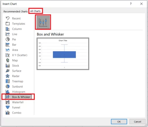
1. 3. This will launch the Charts dialogue box as follows. Go to All Charts.
   4. Select ʻBox & Whiskerʼ chart from the pane on the left.

1. 5. Click Okay to have the chart inserted.

 

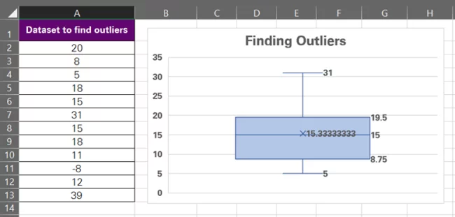
What’s best about the Box & Whisker chart is that it includes some outlier stats within the chart. Note the highlighted values below – those are Q1 and Q3.

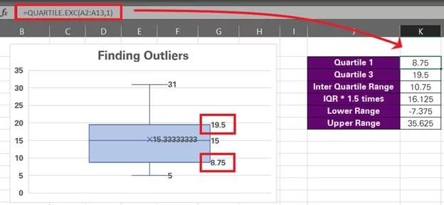
To help you double-check the quartile values on the chart, we have calculated Q1 and Q3 for this data set using the QUARTILE.EXC function. And the values match (8.75 and 19.5)

Similarly, following the same IQR rules, we have calculated the outlier limits for this data set that turn out to be -7.375 and 35.625.

You don’t have to calculate these manually. The box and whisker chart will plot the outliers for you. We have calculated these numbers only to help you know what runs on the back of the box and whisker plot. Also, to prove a point that’s just about to come.

Pro Tip!

The top and bottom point of this chart is meant to show the minimum and maximum values of the data set that are not an outlier.

 

However, a closer look into the data will reveal that the minimum and maximum values of our data set are 39 and -8. But the plot shows them as 31 and 5. Why? You’ll know that once we have the outliers plotted on our chart.

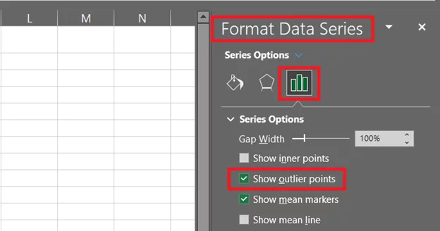
1. 6. Now to have the outliers spotted, click on the box and whisker plot, and a Format Pane will launch to the right of your sheet.
   7. From this pane, go to Series Options > Show Outlier Points.

 

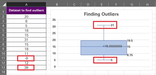
1. 8. With this, the box and whisker chart begins to show two blue dots on the top and bottom that specify the outliers for your data.

 

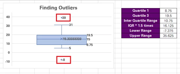
Coming back to the question we raised only two steps ago – why does the chart show 5 and 31 as the minimum and maximum values when the smallest value from this data set is -8 and the largest 39?

That’s because both these values, -8 and 39, go beyond the outlier threshold of -7 and 35.625. Hence, the blue dots show the outliers, and these numbers are not covered within the minimum/maximum range of the data set.

That’s how you can find outliers using a Box & Whisker chart without having to calculate it first.

Note!

The Box & Whisker chart has a predefined criterion for identifying outliers, i.e. values that exceed 1.5 times the IQR of a data set. This makes it a quick method for detecting outliers in Excel, but at the same time, limits it down, too.

For instance, if you have a different criterion for identifying outliers (like the standard deviation method, or the Z-Score method, or 2 times the IQR, etc.), the Box & Whisker plot won’t help you in identifying outliers per your criterion.

Scatter Plot

Another way you can visualise outliers in Excel is by plotting an XY Scatter chart.

Here’s how:

1. 1. Select the data to be visualised in an XY Scatter chart.

1. 2. Go to the Insert tab > Charts Group > Recommended Charts.

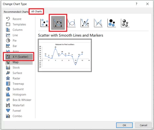
1. 3. This will launch the Charts dialogue box as follows.
   4. Go to All Charts.
   5. Select the ʻXY (Scatter)ʼ chart from the pane on the left. Select the further chart type that has smooth lines and markers (makes detection easy).

 

1. 6. Click Okay to have the chart inserted.

 

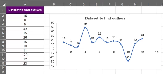
The next step is to scan the chart carefully to find the odd points, and it doesn’t need a lot of effort to see two data points that outdo the entire chart, i.e. -28 and 49.

 

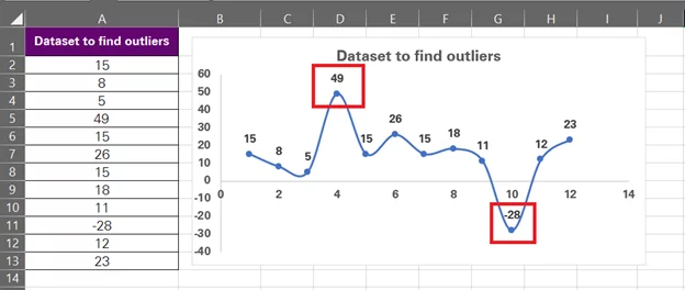
That’s how XY scatter charts help you identify outliers. Instead of scanning through the details of the data, you have it pictured in front of you so you can pick out whatever seems unusual.

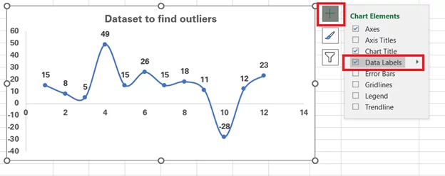
Note: If your scatter plot doesn’t show data labels (the values for each marker), don’t worry. Click anywhere on the chart to select it > Click on the plus icon to the right > Check the option for ʻData Labelsʼ.

Handling Outliers Once Detected

Once you’ve identified the unusual data points messing with your data, what’s next? You need to handle these. There are different ways you can address, correct, or manage outliers in a data set.

Let’s consider these options:

1.    Removing Outliers

If you believe the outliers in your data are irrelevant to your analysis or are a product of data entry errors, you can simply remove them.

And it’s pretty simple to do that. For example, we have identified the outliers in this example by using the formula above.

Now, since we plan on removing them, you can filter them by applying data filters:

Note: I do understand this sounds a little odd when two outliers can be deleted just like that, but let’s just assume this is a long, long list, and it’s arduous to delete each outlier manually.

1. 1. Select the column header where you have the outliers identified. Column B for us.
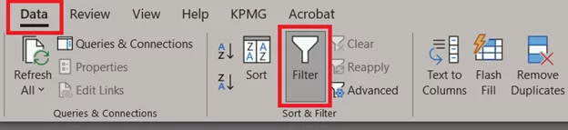
   2. Go to the Data tab > Sort & Filter > Filter.

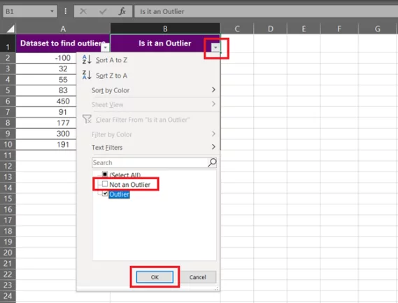
1. 3. See the small drop-down menu button on the column header. Click it.
   4. Uncheck ʻNot an Outlierʼ and press Okay.

1. 5. And you’d have the outliers filtered only.

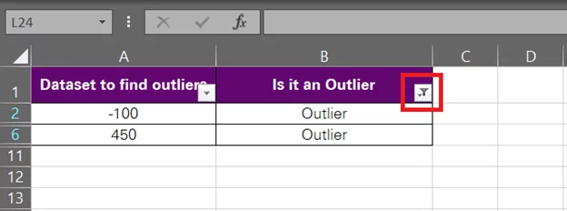
1. 6. Select them and delete them (delete the entire row or just these values manually – however you like it).
   7. Remove the filters from your data by going to the Data tab > Sort & Filter > Filter.

There you have it – clean and crisp data with no outliers.

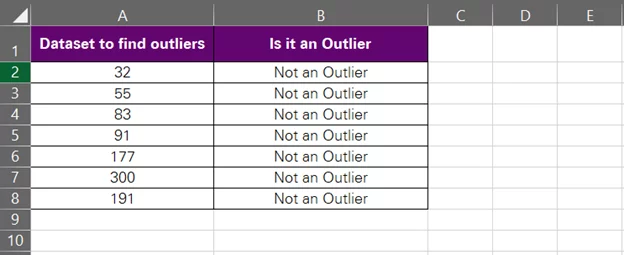
Check out how we’ve deleted the outliers from this data set here.

Interesting? Learn more about the advanced filters of Excel here.

Careful!

You must only opt to remove outliers from a data set when you’re sure they are not needed, are irrelevant, or it’s fine to have them removed. Also, to be on the safer side, it is suggested to keep a copy of the original data (including outliers) before you go ahead with the deletion.

It is important to be cautious with this step as it might lead to data loss. Be sure to have a clear rationale for eliminating the outliers this way.

2.    Replacing Outliers

Another solution to help outliers is to replace them, and there are several ways to do it.

Transform Data

You can mathematically transform the data to make it more normally distributed and reduce the distortion caused by outliers. Some common transformation methods include natural logarithm, taking the square root, or Box-Cox transformations.

Doing so will reduce the impact of the extreme values and make the data distribution less skewed.

Winsorizing

By Winsorizing your data set, you can cap the extreme values by replacing them with the nearest non-outlier values.

You can calculate a certain acceptable percentile (say 95th or 99th) for your data set. Any values that exceed this percentile can then be replaced by the value at that percentile.

For example, here we have a data distribution:

8, 9, 11, 13, 15, 16, 17

Let’s set the cap to the 98th percentile.

The 98th percentile for this distribution is 16.88 (calculated through the PERCENTILE.INC function of Excel).

To Winsorize this data set, we will look out for any values that exceed 16.88 (which is only 17) and replace them with 16.88 (the 98th percentile). So, the data set becomes:

8, 9, 11, 13, 15, 16, 16.88

That’s one way you can replace outliers in a data set.

Data Truncation

With the data truncation technique, you can set up a threshold and replace any values above or below that threshold with a specific value (within the threshold). You’d commonly see this happen in finance, where extreme values may be capped up to a specific limit (e.g. stock prices above or below a certain value).

Imputation

Instead of removing outliers, you can wear the cap of a statistician and impute their values with statistical methods. Draw reasonable estimates based on the rest of the data, such as the mean, median, or a regression-based approach, and replace the outliers with them.

Careful!

You can use these and many more methods to stabilise the data distribution in question, but to reach optimal results, a lot of caution needs to be exercised. While these transformations can help minimise the impact of outliers and make the data more amenable to standard statistical methods, the outliers are never entirely eliminated. They may still exist in the data with a reduced impact.

Having said that, you must pay attention to the data stabilisation technique you choose. What goes best for your data set will come from the nature of the data.

3.    Retaining Outliers

Removing or replacing outliers is not always the solution. Sometimes, you might want to keep outliers and focus on them.

When outliers are considered as noise or anomalies, they can sometimes provide valuable insights and be useful for research in various fields.

For example, outliers in medical stats can be representative of rare but critical cases. Like in clinical trials, outliers may indicate that a treatment has an exceptional effect on a small subgroup of patients. Identifying these outliers and digging them down could lead to the development of more targeted and effective treatments.

By retaining outliers, you acknowledge their presence in the data set while ensuring that they are appropriately captured by the statistical measures or models you employ. This approach can be useful when you believe that the outliers may contain valuable information or when you want to avoid data loss.

Advanced Tips And Tricks

If you want to play around like a pro, you can always resort to advanced techniques to manage outliers. Such as deploying Excel add-ins and VBA.

Using Excel Add-Ins Or Tools For Advanced Outlier Detection:

Advanced outlier detection techniques will often require more specialised tools, particularly add-ins in Excel. Here are some of the Excel add-ins that you can explore for advanced outlier detection in Excel.

Data Analysis ToolPak:

One commonly used Excel add-in is the Data Analysis ToolPak. This add-in provides various statistical analysis tools, including regression, correlation, and hypothesis testing.

We are, however, going to use it for quick outlier detection using the Z-score method.

Here’s the data set that we’re going to track down for outliers using the Z-score method.

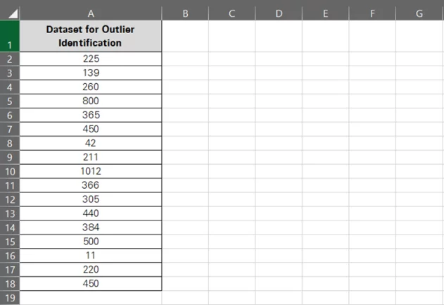
Let’s use the Data Analysis ToolPak to pick outliers from this one.

1. 1. Go to File tab > Options.
   2. Within the Options window, select ʻAdd-insʼ from the left pane.
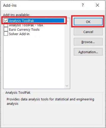
   3. Select Analysis ToolPak and click on the ʻGoʼ button at the bottom.

1. 4. Check the box for Analysis ToolPak and click Okay.

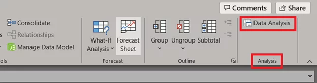
1. 5. This will add a new group of buttons to the Data tab on the Ribbon.

Pro Tip!

All the above steps are only relevant if you do not have the Analysis ToolPak add-in enabled already.

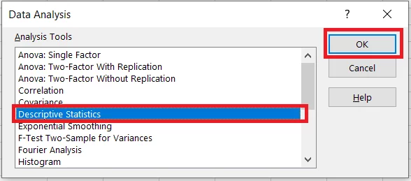
1. 6. Go to the Data Tab > Analysis Group > Data Analysis.
   7. From the dialogue box that opens next, select Descriptive Statistics > OK.

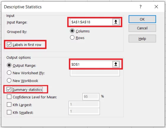
1. 8. In the Descriptive Statistics dialogue box, select the input range as A1 to A18 (wherever the data for outlier detection lies).
   9. Check the option ʻLabels in the first rowʼ as we have a header there.
   10. Choose where you want the output to be displayed. We are setting it to cell D1 in the same sheet.
   11. Check the button ʻSummary Statisticsʼ and hit okay.

Excel will produce a descriptive statistical summary for the given range of data. Observe closely to note that it contains the mean, standard deviation, median, and even the skewness degree of the data.

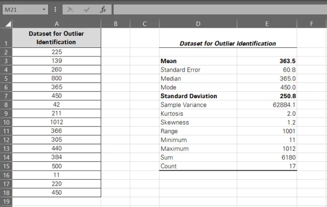
All of this with just a single operation – having all these stats calculated otherwise would have taken quite some time and a range of functions.

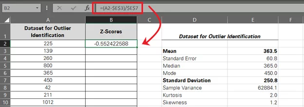
1. 12. To find outliers for the data, let’s employ the Z-score formula for each value as follows:

Z Score = (Value – Mean) / Standard Deviation

To make a formula out of it using cell references, here’s what we’d do:

= (A2 – $E$3) / $E$7

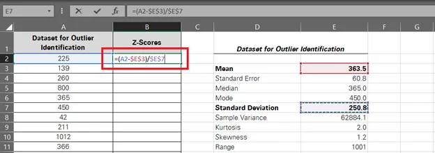
Note that we have used a relative reference for the value (A2) so that we can drag and drop the formula. The absolute references for the mean and standard deviation will remain the same.

1. 13. Hitting ‘Enter’ calculates the Z-score for the first data point.

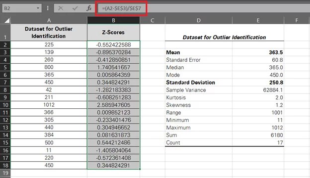
1. 14. Drag and drop the same to the whole set to have the following results.

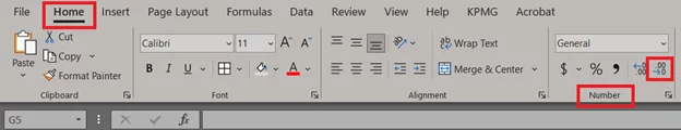
1. 15. Adjust the decimal points to zero by going to the Home tab > Number group > Decimal adjustment.

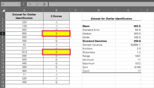
Normally, an outlier would be a data point whose Z-score is +-2, +-3, or beyond. However, this is something entirely subjective, and you can set the threshold yourself.

Z-scores indicate how many standard deviations a data point is from the mean. The bigger the difference, the higher the chances of that data point being a potential outlier.

1. 16. Identify potential outliers by examining the Z-scores.

Or you can apply filters to pick them out like this.

Other Add-ins

In addition to the Data Analysis Toolpak, there are many other and more advanced Excel add-ins that you can leverage to find outliers in Excel.

For example, XLSTAT is a popular Excel add-in for advanced statistical analysis. It offers a range of outlier detection methods, like Mahalanobis Distance, Grubbs’ test, and multivariate outlier detection techniques.

It helps you perform in-depth outlier analysis and visualise the results.

Similarly, StatTools is another Excel add-in that contains a library of advanced statistical tools, including outlier detection methods like Dixon’s test and generalised extreme Studentized deviate (ESD) test.

These methods allow for more sophisticated outlier identification and handling.

And the list goes on.

Automating Outlier Detection Using Excel Macros Or VBA:

Apart from Excel add-ins, you can also use Excel macros or run a VBA script to perform automatic outlier detection in Excel. Here are some ideas on how:

Custom Functions:

VBA allows users to create custom functions for outlier detection. These functions can be designed to implement specialised outlier identification methods or to automate existing ones.

You can create and use these functions directly in your Excel worksheets.

Using VBA scripts, you can also create user-defined functions that can be used in Excel formulas. If proficient enough, you can write your own VBA code to define your outlier detection algorithms and then use them like built-in Excel functions. Or you can always seek help from an expert to write you a code that fits your needs.

Automate Data Preprocessing:

You can record macros to sort your data and run them on every new set of data to automate data preprocessing tasks, such as data cleaning and transformation, before performing outlier detection. This ensures consistency and efficiency in your analysis.

Interactive Dashboards:

Using VBA, you can also create VBA-powered interactive dashboards that allow you to visualise and explore data with advanced outlier detection methods.

With these, you can interactively adjust outlier detection parameters and thresholds. Not only that, but you can also schedule regular outlier detection processes through VBA. This can help monitor data streams and automate the identification of outliers in real time or at specified intervals.

MS Excel lays down a good foundation for basic outlier detection. However, if you’re keen to explore more advanced and specialised techniques, there’s no harm in checking out advanced Excel add-ins, tools, and custom solutions using VBA.

VBA is much more powerful than you think! It can help you streamline the outlier detection process by making it more efficient and tailored to your specific analytical needs.

Advantages And Disadvantages Of Using Excel For Outlier Detection

We’ve delved quite deep into the world of outliers, from knowing what they are to calculating them, to detecting them, and to handling them.

But why through Excel? Not that you cannot play around with outliers without Excel, but using Excel to identify and handle outliers brings significant advantages to the table. We describe them below.

Flexibility & Ease of Use

Who doesn’t know about Microsoft Excel? It was built to be a user-friendly and widely accessible tool for all grades of users (beginners to pros).

We demonstrated through various examples above that you don’t need to be too big of an Excel whiz to perform basic outlier detection using this software. The possibility of using built-in functions and simple formulas to calculate, detect, and handle outliers makes Excel a versatile choice for many users out there.

Outlier Visualisation

Excel is an all-in-one spreadsheet program. It has a wide variety of charting and graphing tools to offer that not only allow you to plot your data but also to visually inspect your data for outliers.

There’s a wide variety of charts available in Excel that you can create to picture your data and scan potential outliers.

Built-In Functions

In the examples above, it took us a handful of functions to find outliers for our data sets. Starting from functions like QUARTILE, AVERAGE, and STDEV, to PERCENTILE and so much more – Excel makes outlier detection much easier.

Excel built-in functions prove super valuable for calculating summary statistics and identifying potential outliers based on whatever criteria you choose.

Customise your Formulas

And in case you don’t have a stipulated function for something, you can always tweak a pair of functions to reach your desired results.

Excel’s formula language allows for a high degree of customisation. Also, once you have customised a formula, Excel 365 allows you to create your very own function out of it through the LAMBDA function.

 

With a great deal of advantages comes a fair share of disadvantages of using Excel, too. Stay alert to the following aspects of using Excel for outlier detection.

Size Limitations

Excel has a total of 16,384 columns and 1,048,576 rows in a worksheet – while this may sound like a lot, let me tell you it’s not.

When talking about huge data sets and hefty extractions, Excel often fails to serve enough. This limits the use of Excel in handling very large data sets. More so, if tested to its limits, you can expect Excel to run slow and fail at supporting extensive data cleaning and outlier analysis for massive data sets.

Lack of Automation

Excel is not the best choice for automated complex outlier detection processes. If you get to deal with such huge data sets more often, you may need to repeatedly perform manual outlier detection operations, which can be time-consuming and mundane.

Finding outliers and handling them using Excel involves a variety of steps and functions, and it may not be smart to continue repeating them over and over again.

Complex Outlier Criteria

Putting aside the simple mathematical and statistical methods for finding and detecting outliers, Excel’s built-in functions may not be sufficient for handling complex outlier criteria (if any).

To help such a situation, users may need to implement custom VBA scripts or resort to other specialised spreadsheet software.

Can’t Run Advanced Statistical Techniques

As a data set continues to grow, the efficiency of Excel sees a slump. Apart from the common functions and formulas, it may not offer all the advanced statistical techniques needed for robust outlier detection. For example, multivariate outlier analysis can only be done using specialised statistical tools.

Data Loss & Unreliable Results

We don’t blame MS Excel for that because it was never meant to be a very robust spreadsheet software when it comes to data protection. There are many easy ways to break into apparently locked spreadsheets, and Excel is not a sensible choice to make when you’ve got sensitive data on your hands.

Also, if you resort to removal as a means of handling outliers, know that manual removal of outliers may result in data loss, which can be problematic. Particularly when outliers are indicative of rare but essential cases or otherwise contain valuable information.

Last but not least, relying solely on Excel’s visualisations for outlier detection may lead to errors in identifying outliers and subjective inferences.

In short, there is no doubt about the fact that Excel is a valuable tool for basic outlier detection. It offers flexibility and is one of the easiest spreadsheeting software to use.

However, it only makes a good choice for small to medium-sized data sets with a basic outlier criterion. For large and complex data sets that need advanced level outlier detection techniques in place, it’s advisable to look out for more specialised statistical software. Or even programming languages like R or Python.

Best Practices

There always exists room for improvement in everything you do. Below, we have a list of some best practices that you can adopt to ensure better outlier detection.

Ensuring Data Integrity Before Outlier Detection:

No matter how robust or advanced measures you put in place, it’s of no use unless you’re sure about the integrity of the data at hand.

Before you sift through your data distribution to pick outliers, check if it’s free from errors. The degree of error you can expect in your data depends upon the entry/import methods applied to it. To take the safer side, ensure to have addressed any missing values, duplicates, and inconsistent formatting issues beforehand. More like data cleaning.

Examine the data for potential data entry errors and inconsistencies. Once done, validate the data against domain knowledge or external sources.

Perform appropriate data transformations (like scaling or normalisation) to prevent distortions. See to it that data preprocessing is done consistently and transparently.

Regularly Updating And Reviewing Outlier Criteria As Data Evolves

Unless you have an automated outlier detection method in place, be mindful of the fact that as the data changes over time, new outliers may emerge, or old ones may lose significance. Perform a periodic review of your outlier criteria to adapt to changing data patterns.

A value that makes an outlier for your data set per one method may not be an outlier for the same data set under another method. And since this is a purely subjective matter, it’s fine. Clearly define the criteria for what constitutes an outlier. Document these criteria and update them as necessary.

Taking outlier detection to broader levels, it is always advisable to automate the outlier detection process in Excel. This makes it easier to apply updated criteria and keep your analysis accurate.

Collaborating With Domain Experts To Understand The Significance Of Detected Outliers:

Outlier identification is a whole science. Work closely with subject matter experts who understand the context of the data. They can provide valuable insights into advanced-level outlier detection and help differentiate between meaningful anomalies and data errors.

Lastly, remember that feedback is a continuous process. Establish a feedback loop with experts to continuously improve your outlier detection process. This will help you refine criteria and identify areas where outliers offer valuable information.

Why Is It Important To Follow These Practices?

Employing some or all of the above-mentioned practices will help you handle large data sets with ease and accuracy – and guess what? These practices help outlier detection on so many levels.

Outlier detection is an iterative and collaborative effort that involves not only data analysis but also domain expertise. By maintaining data integrity, keeping criteria up to date, and getting in touch with subject matter experts, you can ensure that all outliers are properly identified and interpreted.

Conclusion

We are in the last quarter of 2023 and officially in the realm of data analysis.

Identifying and managing outliers is not a choice; it’s fundamental to ensure your data is in the right shape and that the inferences you draw are accurate and reliable.

Outliers can not only distort statistical measures, but they can also skew visualisations and lead to misguided conclusions. To have your results sorted, make sure you approach outliers methodically and thoughtfully.

The tutorial above explains several ways you can leverage Excel to hunt down outliers in a given data set. Practising these can help you harness the full potential of your data and make informed decisions like an expert.