Excel’s LAMBDA Function [Simple Breakdown]

The LAMBDA Function lets you create and modify your own formulas.

Instead of creating complex sets of formulas with messy referencing, just master this one skill!

We will guide you through the basics of the function, and show just how it can save your time.

We find many delegates on our Excel intermediate course have also never heard of this function!

What Is The Excel Lambda Function?

It enables users to create custom functions that they can save by any name they want.

This function will then be saved and can be used throughout the workbook.

You can now compose any formula in Excel, wrap it into the LAMBDA function, give it a suitable name and save it as a function.

The next time you need to apply the same formula, don’t go all the way retyping it.

You can instead refer to the custom function built and saved by you previously.

And the good news! You don’t need to be a programmer or VBA specialist to do all of this.

Mastering this tricky skill will take you from average to an expert in Excel.

Syntax and Arguments

The Excel LAMBDA function reads as follows.

= LAMBDA ( [parameter_or_calculation], [parameter_or_calculation],.. )

• Parameter: Whenever you type any function, a small popup shows you the number of arguments a function has and that you must enter for the function to run.

This time it’s you who wears the developer’s hat. Parameters define the arguments that you want to set for your formula.

A parameter is an input value that can be in the form of cell references or values. Excel can accept up to 253 arguments.

• Calculation: This has to be the formula that you want to be converted into a function.

Let’s jump right into the article to see how you can create your very own function.

How To Create The Excel LAMBDA Function

It’s time we create our function.

Step 1: Write the LAMBDA function in Excel

• • Make a core formula. The LAMBDA Excel function is a formula instilled into Excel by the name of a function.

For example, if you want to divide two numbers in Excel, you write the following formula.

= 20 / 5

It involves no function and is a simple formula. Run this in Excel, and you’d get the following answer.

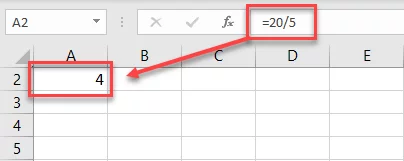
The answer is 4. Simple.

So our formula is 20 (the dividend) divided by 5 (the divisor).

Dividend / Divisor

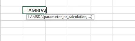
• • Launch the LAMBDA function to create your function

= LAMBDA (

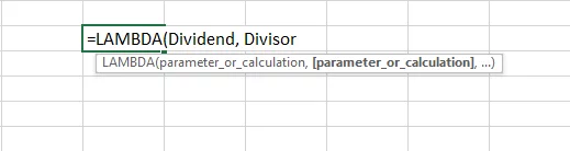
• • Define the parameters (arguments).

These are the input values that would be required whenever the targeted function is run. We want our function to have two input values, the dividend, and the divisor.

• • Write both these as the arguments of the LAMBDA function.

= LAMBDA ( Dividend, Divisor,

• • Next, define the calculation (the formula).

Our core formula is dividend/divisor. Add another comma to the LAMBDA function to define the said formula.

= LAMBDA ( Dividend, Divisor, Dividend / Divisor )

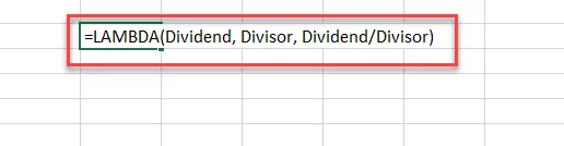
The Excel LAMBDA function is all complete and set to go.

Don’t hit ‘Enter’ already. Or if you do, Excel will return a #CALC! error because it has no values to process.

Step 2: Test the LAMBDA functions

Has Excel rightly picked the function defined above? There’s one way how you may check this.

The ‘function call’ allows you to check if the formula defined in the LAMBDA function works correctly.

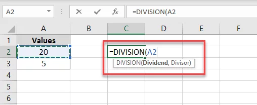
1. • To test the LAMBDA function, give it some input values right after the parenthesis is closed.

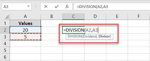
= LAMBDA ( Dividend, Divisor, Dividend / Divisor ) (A1, A2)

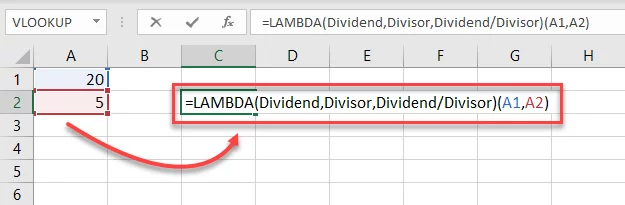
We have added a new parenthesis to the end of the LAMBDA function (A1, A2).

The LAMBDA function will test the formula (Dividend / Divisor) using these two cell references.

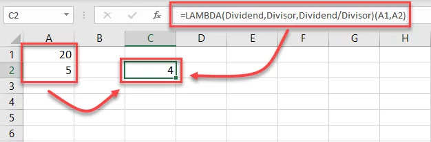
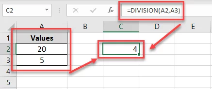
The answer is 4 which is 20 divided by 5. The results provided by LAMBDA adhere to the result of the simple formula (= 20 / 5).

It is always good to test your LAMBDA function to ensure everything sits in place.

Step 3: Save the function

We have created and tested the LAMBDA function in Excel already. Now it’s time to name it and save it in Excel.

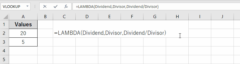
• • Copy the LAMBDA formula. Make sure to only copy the following part of the LAMBDA formula.

= LAMBDA ( Dividend, Divisor, Dividend / Divisor )

Must not copy the function call. It is only meant to test the function and has nothing to do with saving the function.

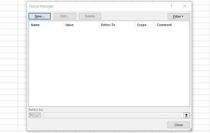
• • Go to Formula > Defined Names > Name Manager. Or use the keyboard shortcut [Control Key + F3] to launch the Name Manager.

• • This launches the name manager as shown below.

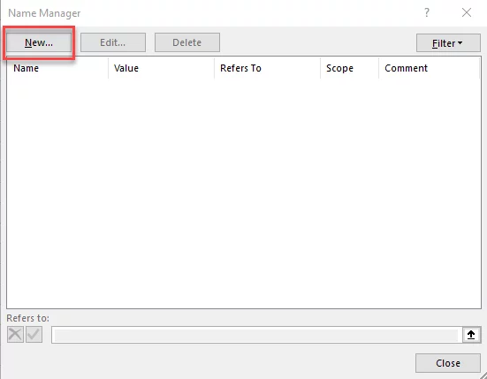
• • From the Name Manager dialog box, Click ‘New’ as highlighted above.
  • In the Name Manager, fill in the following fields:

1. 1. 1. Against the Name box, type a suitable name for the function. We are setting it as DIVISION.
      2. Against the Scope box, choose ‘Workbook’. This means you can use this function across the whole workbook. Alternatively, if you select a particular Sheet as the scope, you’d only be able to use this function across that sheet.
      3. Against the Refers box, paste the formula copied above. The formula must start with an equal sign (=). To make any changes to the formula once pasted, press the F2 key to enter the editing mode.

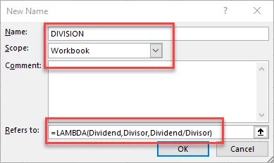
• • Click ‘Okay’ to save it.

Testing the function!

Guess what? We are all done. It’s time we test the function we’ve just created.

• • Activate a cell and begin writing with an equal to sign:

= DIVISION (

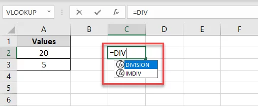
Must Note!

Did you notice something? As soon as you typed the first three letters of DIV, Excel identified it as a function. This means the DIVISION function is now saved to the Excel functions library. Using a custom function after it’s created in Excel is seamless enough.

• • The first argument of the DIVISION function is ‘dividend’.

= DIVISION ( A1

We have created a reference to cell A1 as the first argument it contains the number to be divided.

• • The second argument of the DIVISION function is ‘divisor’.

= DIVISION (A1, A2)

We have created a reference to cell A2 as the second argument contains the divisor.

• • Hit ‘Enter’ to see the results as follows.

Excel runs the division function as intended i.e. Dividend / Divisor.

That’s how you can create and save any function in Excel.

Things to Remember about the LAMBDA function

To have a seamless experience creating and running functions with the LAMBDA function, take note of the following:

1. 1. The function or parameter name must not be longer than 255 characters.
   2. It must not start with any punctuation mark except for an underscore ( _ ) or backslash ( \ ).
   3. Do not use names that coincide with the names of built-in Excel functions.
   4. Do not use names that are similar to cell references like AAB1 etc.
   5. Must not enter more than 253 parameters into a single LAMBDA function.

Lambda Function Examples

We are already across one basic example of creating a function in Excel using LAMBDA.

Rest is all about practice. By introducing the LAMBDA function, Microsoft Excel has set forth limitless opportunities for Excel users to create functions.

Let’s see some more examples of how you can create amazing functions in Excel which you always thought should’ve been there!

Example No. 1: Basic Formula

Remember the formula for finding the area of a right-angled triangle? No?

Neither do we. Let’s feed it into Excel as a function so that the memorizing responsibility shifts to Excel.

We find this example is great on our advanced courses.

Step 1:

• • The formula for finding the area of a triangle is as follows:

= (b*h) / 2

B = Base of the triangle; and

H = Height of the triangle

• • Launch the LAMBDA function to create your function

= LAMBDA (

• • Define the parameters (arguments). So our core formula has two parameters and is:

= (Base * Height) / 2

• • Let’s formulate this into the LAMBDA function.

We want our function to have two input values, the base, and the height.

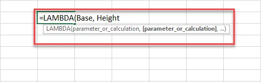
• • Write both these as the input parameters of the LAMBDA function.

= LAMBDA ( Base, Height,

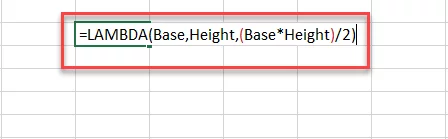
• • Next, define the calculation (the formula).

= LAMBDA ( Base, Height, (Base*Height)/2 )

The LAMBDA function is all complete and set to go.

Step 2:

Time to test the LAMBDA function!

1. • Give it the input values for base and height right after the parenthesis is closed.

= LAMBDA ( Base, Height, Base / Height ) (A2, B2)

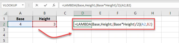
• • The LAMBDA function will test the formula (Base*Height / 2) using the values in Cell A2 and B2.

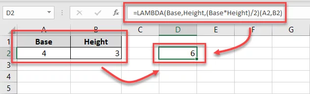
The answer is 6. The result provided by the TAREA function adheres to the result of the simple formula (= (4*3)/2).

This means we are all good to go.

• • Copy the following part of the LAMBDA formula.

= LAMBDA ( Base, Height, Base / Height )

• • Go to Formula > Defined Names > Name Manager.
  • This launches the name manager as shown below.

• • From the Name Manager dialog box, Click ‘New’ as highlighted above.

• • In the Name Manager, fill in the following fields:

1. 1. 1. Against the Name box, type a suitable name for the function. We are setting it as TAREA.
      2. Against the Scope box, choose ‘Workbook’.
      3. Against the Refers box, paste the formula copied above.

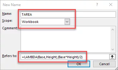
• • Click ‘Okay’ to save it.

Step 4:

And we are all done. Let’s test the function we’ve just created.

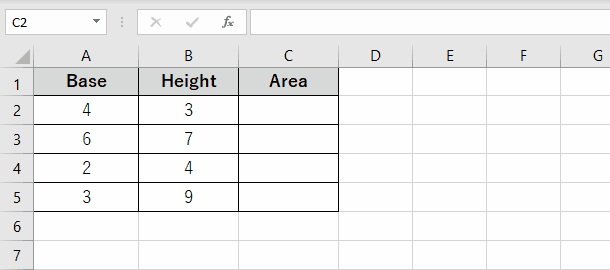
Here we have some data points for the base and height of a triangle.

• • To find the area using these data points, activate a cell and begin writing with an equal to sign:

= TAREA (

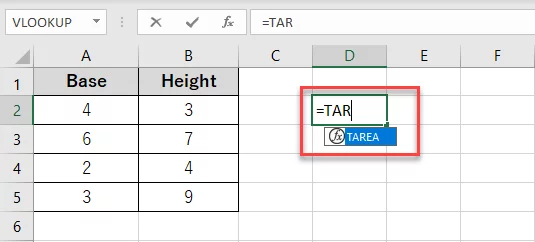
As soon as you type the first few letters, Excel identifies it as a function.

• • The first argument of the TAREA function is ‘base’.

= TAREA ( A2

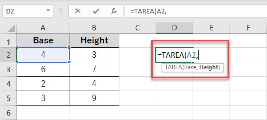
We have created a reference to cell A1 as the first argument it contains the bases.

• • The second argument of the TAREA function is ‘height’.

= TAREA (A2, B2)

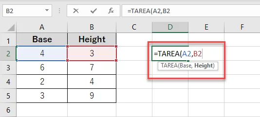
We have created a reference to cell B2 as the second argument contains the height.

• • Hit ‘Enter’ to see the results as follows.

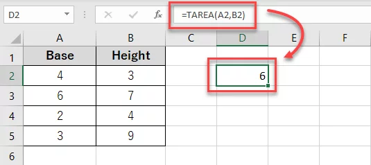
Viola! Excel runs the TAREA function as intended i.e. (Base*Height) / 2.

With this, you now have your function for calculating the area of a triangle in Excel.

Pro Tip!

Unlike ordinary functions, as you begin typing a Custom Lambda, Excel won’t show a descriptive text for the function. For in-built functions, this short text explains what the function is meant to do.

To help this, write a descriptive text for the function in the Comment box of the Name manager. This text will appear with the formula every time you use it in Excel.

Example 2: Multiple parameters

Until now, we have seen examples of creating a custom LAMBDA function with two parameters only. However, the maximum number of parameters that a LAMBDA function can have is 253.

Let us now customize a LAMBDA function with more arguments (but not 253 obviously).

The image below shows the data for the employees of a Company.

The data includes details like the joining and leaving date of employees, their salary, and deduction percentage.

How do we calculate the amount of their gratuity?

The formula for calculating gratuity is as follows:

= (LY – JY) * Salary * (100%-Deduction Percentage)

It has around four input values. How can we set up a gratuity function in Excel for the above formula?

Step 1:

• • Launch the LAMBDA function to create a gratuity function.

= LAMBDA (

• • Define the parameters for your LAMBDA function.
  • Our formula for gratuity has four parameters:

1. 1. 1. Joining Year (JY)
      2. Leaving Year (LY)
      3. Salary
      4. Deduction percentage

• • Write all the above four input values as parameters of the LAMBDA function.

= LAMBDA (JY, LY, Salary, Deduction,

• • Next, define the calculation argument (the formula).

= LAMBDA (JY, LY, Salary, Deduction, (LY– JY)*Salary*(100%-Deduction))

We have defined the calculation with all four input values.

Pro Tip!

If your formula has more than one operation performed, ensure using parenthesis in the right place.

The operation that you want to be performed first must be enclosed in parentheses. If you miss out on the parenthesis, Excel will perform the operations in the PEMDAS order.

PEMDAS stands for Parentheses, Exponents, Multiplication, Division, Addition, and Subtraction.

Step 2:

• • To test the LAMBDA function, give it the input values for all four parameters.

= LAMBDA (JY, LY, Salary, Deduction, (LY – JY)*Salary*(100%-Deduction)) (B2, C2, D2, E2)

Here comes the testing phase.

The LAMBDA function computes the gratuity payment as follows:

The answer is $88,000.

Let’s double-check the same by applying the formula separately in Excel.

The answers match! Good to go.

• • Copy the following part of the LAMBDA formula.

= LAMBDA (JY, LY, Salary, Deduction, (LY– JY)*Salary*(100%-Deduction))

• • Go to Formula > Defined Names > Name Manager to launch the name manager.

• • In the Name Manager dialog box, fill in the following fields:

1. 1. 1. Against the Name box, set the name of the function as ‘GRATUITY’.
      2. Against the Scope box, choose ‘Workbook’.
      3. Against the Refers box, paste the formula copied above.

• • Click ‘Okay’ to save it.

Let’s test the function we’ve just created using the same dataset.

To find the Gratuity payment for employee A, activate a cell and begin writing:

= GRATUITY (

• • For each parameter of the GRATUITY function, refer to the relevant cell from the given data.

= Gratuity (B2,C2,D2,E2)

• • • Where Cell B2 contains the joining year.
    • Cell C2 contains the leaving year.
    • Cell D2 contains the salary of each employee.
    • Cell E2 contains the deduction percentage.

• • Hit ‘Enter’ to see the results as follows.

Here we have the gratuity for Employee A. Drag and drop it to the remaining employees to find the gratuity payment for them all.

Pro Tip!

Besides all the good that the LAMBDA function has to offer, it is only restricted to a single workbook. With all due regret, this means you have to create a custom function for every workbook. These are not reusable functions.

An easy way to copy the LAMBDA function from one book to another is – copying a sheet from that workbook (that contains the custom function) to the new workbook.

Example 3: Embedding other functions in LAMBDA

Have you ever calculated the average in Excel using the Average function of Excel?

Easy, right? However, if you have ever happened to calculate the weighted average in Excel, you’d know Excel doesn’t offer any inbuilt function for it.

You need to set up a formula to calculate the weighted average. Or else, you might have to use a combination of other functions to calculate the weighted average. If Excel lacks a function, let’s create one for ourselves. And here we go!

The image below shows the data for an investment portfolio.

The data includes the share prices of three different companies. And the number of shares held in each company.

Can we calculate the weighted average share price for this portfolio?

The core formula for calculating the weighted average is as follows:

= Sum of all values * Sum of their weights / Sum of weights

In our example, this translates to:

= Sum of Share Price * Sum of No. of Shares / Sum of number of shares

To make it simpler, we can write the above formula in Excel as follows:

= SUMPRODUCT (Values, Weights) / SUM (Weights)

Pro Tip!

The SUMPRODUCT function multiplies any two given arrays and sums the answer.

Need help working with Dynamic Arrays in Excel? Try our guide to the UNIQUE Function here!

Before we make a function for it, let’s try doing it simply in Excel.

We applied the SUMPRODUCT function to multiply the sum of share prices with the sum of the number of shares.

Next, we used the SUM function to find the sum of the number of shares. We divided both the above numbers to find the weighted average share price.

Too gruesome. It’s time we compress this all into a handy function.

If you need more of an explanation on how Arrays work in Excel, we give a breakdown in this article on Cell Array Formulas.

Step 1:

• • Let’s begin writing. Launch the LAMBDA function to create a weighted average function.

= LAMBDA (

• • Define the parameters for your LAMBDA function.

So, we have two input values (parameters) to our LAMBDA function:

1. 1. Values (Share Prices)
   2. Weights (No. of shares)

• • Write the above input values as parameters of the LAMBDA function.

= LAMBDA (Values, Weights,

• • Define the formula for calculating Weighted Average in Excel.

= LAMBDA (Values, Weights, SUMPRODUCT(Values, Weights)/SUM(Weights))

• • To test the LAMBDA function and avoid any #CALC error, let’s populate the function call.

= LAMBDA (Values, Weights, SUMPRODUCT (Values, Weights) / SUM (Weights) ) (A2:A3, B2:B3)

We have referred to two ranges (A2:A3) and (B2:B3) as the Value and Weight of the function call.

The answer is 38.44.

Let’s double-check the same by applying the formula separately in Excel.

The matching answers tell us we are on the right way.

• • Copy the following part of the LAMBDA formula.

= LAMBDA ( Values, Weights, SUMPRODUCT (Values, Weights) /SUM (Weights) )

• • Go to Formula > Defined Names > Name Manager to launch the name manager.
  • From the Name Manager dialog box, Click ‘New’.
  • Fill in the following fields:

1. 1. 1. Against the Name box, set the name of the function as ‘W.AVG’.
      2. Against the Scope box, choose ‘Workbook’.
      3. Against the Refers box, paste the formula copied above.

• • Click ‘Okay’ to save it.

Ready to test the function we’ve just created using the same portfolio data?

• • To find the weighted average share price for this portfolio, write the W.AVG function we just created.

= W.AVG (B2:B4, C2:C4)

> The range B2:B4 contain the values (share prices).

> The range C2:C4 contain the weights (number of shares).

• • Hit ‘Enter’ to see the results as follows.

The weighted average function calculates the weighted average of the shares as 39.30.

A formula that otherwise seemed so long with multiple functions and arguments is now only a matter of two arguments.

Using this very versatile function, you can create custom functions for anything and everything.

Just like the LAMBDA function, other advanced functions of Excel include the XLOOKUP and EFFECT functions. Learn them with us now!

Possible Errors And Troubleshooting

The magnitude of problems that the LAMBDA functions might pose is proportionate to its versatility.

Here are a few common problems you might face with the LAMBDA functions.

1.      Inappropriate Naming:

The LAMBDA functions give you the privilege to set function and parameter names of your choice.

But this comes for a price. You must be careful while you set the names for the function you create. And for the parameters of that function.

For example, if you set the names of the parameters as DIV1, DIV2, and so on, here’s how the LAMBDA function would react.

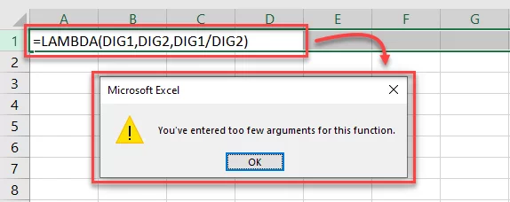
This is because DIV1 and DIV2 are cell references in Excel. When named as a parameter, Excel takes these as a cell reference and not as the name of parameters.

You may change it to something different such as DIVIDEND and DIVISOR.

And Excel wouldn’t pose the error as before.

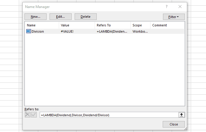
2.      #VALUE! error

If your LAMBDA function gives back a #VALUE error, there could be many reasons for it. Check for either of the following errors:

• • Your LAMBDA function has more than 253 parameters to it. This breaches the maximum limit for the parameters of the LAMBDA function.
  • The names defined for the parameters are not the same as those used in the calculation. This might be a spelling error or an oversight. For example:

= LAMBDA (Dividend, Divisor, Dividand / Devisor)

The parameters defined in the above function have different spelling. However, the names used in the calculation differ in spelling. This will give back a #VALUE error.

• • You have used the wrong number of arguments while using the same function in the workbook.

3.      #CALC! error

With the LAMBDA functions, Excel is likely to pose a #CALC! error if you save the function without testing it by using the function call.

Conclusion

Excel experts call it the most powerful function of Excel – a function that makes Excel Turing-complete.

By introducing the LAMBDA functions, Microsoft has made Excel computationally universal.

At any time, if you find the function library of Excel short for your creative needs, create and add new user defined functions to it.