UNIQUE Function – Mastering Excels Array Tools

There are a number of functions to Excel that enable users to extract a list of distinct values. Ranging from highlighting duplicate values to advanced filters, the methods are many. However, laboring about the same old conventional methods and functions is a thing of the past. The modern Excel Dynamic Array tools allow users to extract unique values with sheer ease and perfection through the UNIQUE function.

The article below must help you learn all that you need to know about it. Get in touch with other Excel courses of ours here.

 

Excel Unique Function

As the name verily suggests, the Excel UNIQUE function is used to extract a range or array of unique values from a given array / range. These values can be text, numbers, time, percentages, dates, or anything.

 

Syntax

Syntax of the unique function consists of three arguments.

= UNIQUE (array, [by_col], [exactly_once])

Arguments

The three arguments offered by the UNIQUE function syntax are analyzed below.

• • Array – This represents the range from where the list of unique values is to be extracted.
  • By_col: This is an optional argument. It specifies if the uniqueness of the values is to be compared by column or by rows. ‘By Column’ equates to 0 or False, whereas, ‘by Row’ equates to 1 or True.

You may set it as 1 (true) or as 0 (false). When omitted, Excel by default takes is equivalent to 0 (false).

• • Exactly_once: This is an optional argument.

If set to 1 (true), it only gives back the items that appear in the data for once.

Set to 0 (false), it returns a list of only the unique values i.e. it eradicates the instances of duplication of data, if any.

If omitted, Excel by default sets this argument to 0 (false).

Return Value

Excel returns an array of all the unique values.

Functions Library

It can be accessed from the Functions library as follows.

Formulas > Functions Library > Lookup & Reference > UNIQUE Function

 

 

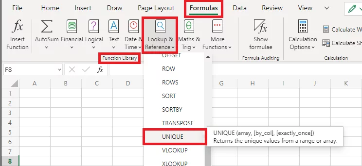
Do note that the advanced UNIQUE function is only available to Microsoft 365 users for Excel 2019 version and above. If you don’t see it in your Functions Library, you probably need to update your Excel.

Know more about the Original 2022 research on Excel Facts and Statistics.

 

Why would someone want to use it?

The Excel UNIQUE function is of much importance as it substitutes all the conventional long-drawn methods of filtering data.

Earlier, Excel users had to deploy methods like highlighting duplicate values and advanced data filter function to pick out unique values. However, now it’s all about putting together the smart UNIQUE function, and your data is all sorted.

Learn about other dynamic array formulas like SEQUENCE function and SORTBY functions here.

 

Unique Use cases

The Excel UNIQUE function can come in handy for a diverse range of purposes. It is an advanced way to extract a list of distinct values from any given data set.

Below are a few reasons why you may want to use it for most of your Excel tasks.

1. As an auditor, you may want to filter our data for data sampling purposes. The UNIQUE function can help you fetch the desired data only through a few clicks.
2. When importing data from the web and other sources, the imported data is often jumbled up and not in very good shape. The UNIQUE function can help with data sophistication of large data sets.
3. This function can also be of help for academic result compilation if you want to filter out students who passed one or more subjects.

The UNIQUE function of Excel can also be of great use to other professions including researchers, statisticians, chemists, etc.

 

Using UNIQUE to return a list of unique values in an array – Basic Example

Taking a look at the example below can help us learn about the basic functioning of the UNIQUE function better.

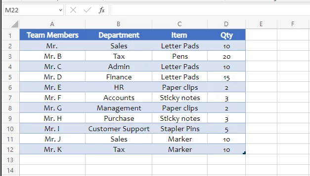
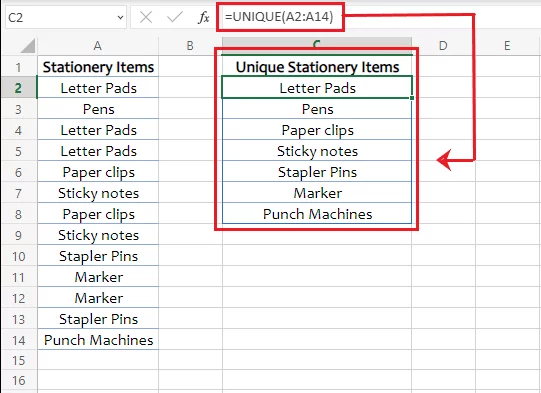
The screenshot below represents records from the procurement department. It shows the purchase requisition raised by team members from different departments.

 

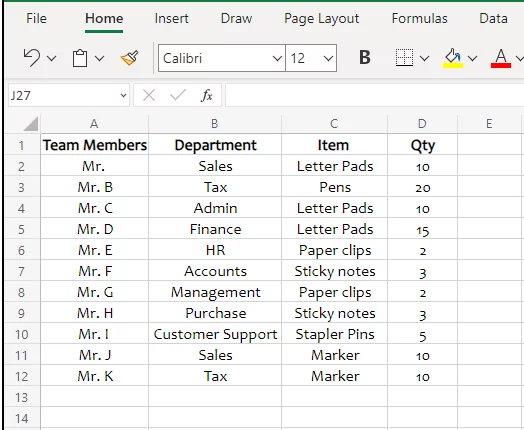
The same stationery item has been requested by multiple team members and appears many times in the list of stationery items.

To derive a list of stationery items to be ordered, you may want to extract a unique list of items. Here’s how you can do it using the UNIQUE function.

 

Step 1:

To extract a list of unique items from the given range, compose the UNIQUE function as follows.

= UNIQUE (C2:C12)

The above syntax is not as simple as it appears to be. Here’s how it is supposed to work.

• • The range is set to C2:C12 which contains the list of stationery items to be filtered.
  • The second argument is omitted as we want the filtration to be done by column. When omitted, Excel by default sets this argument to by_col i.e. 0 (False).
  • The third argument is omitted as we only want a list of unique values. When omitted, Excel by default sets this argument to 0 (False) where a set of unique values is filtered.

The above function can alternatively be composed as follows.

= UNIQUE (C2:C12, 0, 0)

 

Step 2:

After you’ve set up the formula in the cell where you want the unique values to be populated in a columnar shape, hit enter.

 

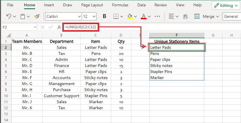
The list produced by Excel contains all stationery items for once i.e. all duplicated values as appearing in the original column are eradicated.

 

More Examples:

You must have found the basic application of the UNIQUE function super simple and easy. It’s time we look into some more examples of applying the UNIQUE function to better learn how it works.

 

1. UNIQUE Function with more than one column/row:

We have seen how the UNIQUE function works to filter out unique values from a single column or row. However, what if the data you want to be filtered is scattered across multiple rows like in the example below?

The image below shows the department code and induction number for different employees. However, the data contains some duplication.

 

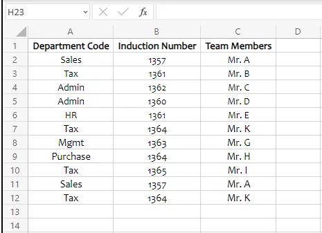
We, therefore, want to filter out a list of unique department codes and induction numbers only. Here is how you can do it.

Step 1:

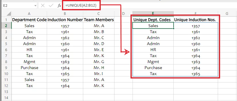
Activate the cell where you want the unique values populated and compose the UNIQUE function formula as follows.

= UNIQUE (A2:B12)

The above syntax is set up as explained below.

• • • The range is set to A2:B12 which contains the department codes and induction numbers to be filtered.
    • The second argument is omitted as we want the filtration to be done by column. When omitted, Excel by default sets this argument to by_col i.e. 0 (False).
    • The third argument is omitted as we only want a list of unique values. When omitted, Excel by default sets this argument to 0 (False) where a set of unique values is filtered.

The above function can alternatively be composed as follows.

= UNIQUE (A2:B12, 0, 0)

 

Step 2:

Hit enter to yield results as follows.

 

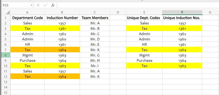
How has Excel extracted the Unique values?

A deeper look into the filtered columns shows that Excel has filtered out only those items that were simultaneously repetitive in both the Columns.

For instance, Tax 1364 appearing in the last row is omitted as the same was appearing twice in the data.

 

 

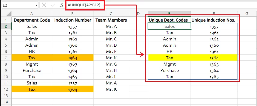
However, ‘Tax’ under Column A appears 4 times, where, in 3 instances, the adjacent induction number is different. The same is therefore not omitted from the unique values.

 

Do you know? Both, the department code and induction number can be combined in one column using the Concatenate function. Learn more here.

 

2. The UNIQUE function applied on an Excel Table

The UNIQUE function from the modern dynamic array functions of Excel is sure to help you extract unique values.

However, how about data that continues to change constantly? To filter out unique values from such a dataset, do you need to reiterate the UNIQUE function over and over again?

Not really! If your dataset undergoes constant updates, you must turn it into an Excel table to have the unique values constantly updated too.

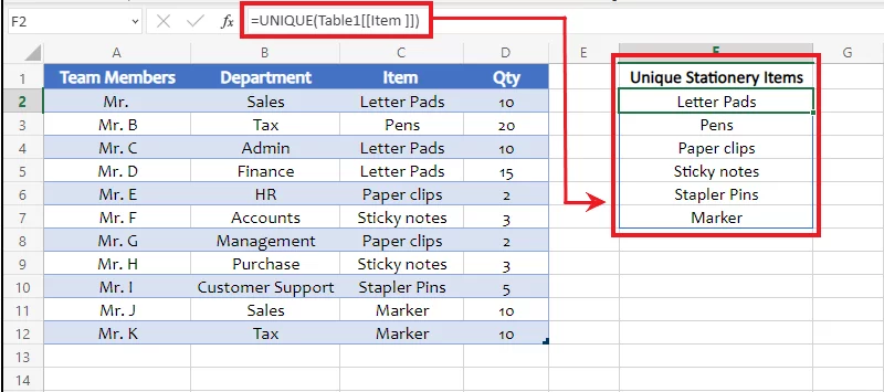
Continuing the same example as above, the image below shows purchase requisition raised by team members from different departments.

 

Before we apply the UNIQUE function to the stationery items listed therein, let’s turn the above data into an Excel table.

Select the data > Insert > Table

 

 

Next, bring the UNIQUE function to action to extract a unique list of the required stationery items.

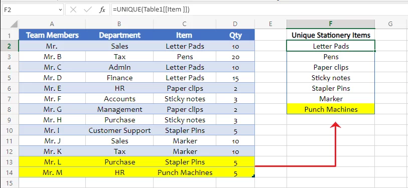
Any updates made to the source data will be automatically reflected in the unique values. Take a look below.

 

 

What has Excel done to the unique values?

When we made updates to the source Excel table, Excel automatically updated the unique values. We added two new items to the source data i.e. Punch Machines and Stapler Pins.

Of these two, ‘Punch Machines’ was not already a part of the stationery items. It is therefore a unique item and is included in the list of unique values.

‘Stapler Pins’, on the other hand, was already included in the stationery items. It is not unique to the source data and is therefore not included in the unique values.

Once you’ve filtered out UNIQUE values, you may switch their layout through the transpose function.

 

3. Nesting the UNIQUE function into the SORT function

After you’ve extracted the unique values from a dataset, what if you want to go a step ahead to sort it in an ascending or descending order?

Simple enough. Both of the said jobs can be performed using the modern Excel dynamic array tools. Go through the example below to learn how.

Step 1:

The data below represents the academic results of different students. However, the data contains a duplication of records.

 

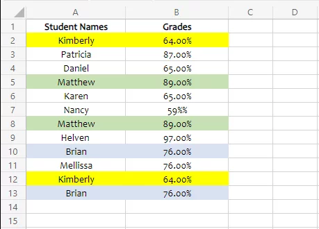
We not only need to extract a unique list of academic records, but the same is then to be arranged in alphabetical order.

To do so, the UNIQUE function is to be set up as follows.

= UNIQUE (A2:B13)

• • • The range is set to A2:B13 as we want a unique set of data extracted.
    • The second argument is omitted as we want the filtration to be done by column which is by default set to 0.
    • The third argument is omitted as we only want a list of unique values to be filtered, which is by default set to 0.

 

Step 2:

After the UNIQUE function is set up, nest it into the SORT function as follows.

= SORT (UNIQUE (A2:B13),1)

• • • The first argument of the SORT function i.e. array is set as the outcome of the UNIQUE function. Once Excel has filtered out Unique values from the source data, we want the same to be sorted in alphabetical order.
    • The second argument i.e. By_array is omitted. As this is an optional argument, Excel assumes it to be the same as the array i.e. A2:B13. This column contains the grades of the students.
    • The third argument i.e. sort_order is set to 1 as we want the names of the students to be arranged in alphabetical order.

 

Step 3:

Hit ‘Enter’ to see results as follows.

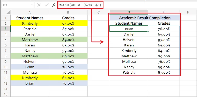
Excel has first filtered out any duplicate values, and only a set of unique values is reproduced in the destination cells using the UNIQUE function.

Next, the SORT function arranges the above set of unique values in alphabetical order.

 

UNIQUE function troubleshooting:

The UNIQUE function is a convenient substitute to the conventional methods for extracting distinct values. Although this function has a relatively straightforward application, you may confront the following problems with the UNIQUE function.

 

1. #SPILL! Error

The unique values sought through the UNIQUE function are likely to take the shape of a row or a column. Taking the example below, the list of unique stationery items is populated by Excel in six cells starting from the cell where the formula is fed under Column C.

 

However, if any of these cells had been populated with any value, the results would have been different.

 

 

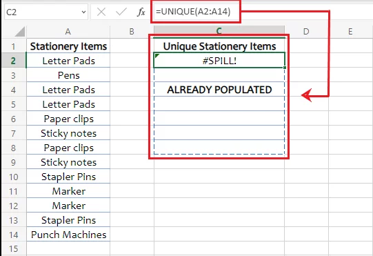
Instead of extracting the list of unique items, Excel gives the #SPILL! Error. This is because cell C4 contains a value already. Delete this value and then enter the formula to resolve the said error.

 

2. #VALUE! Error

Rare, but the #Value! Error is returned by Excel when the formula is not rightly fed. It is usually because of any error made within the composition of the arguments.

To get rid of #VALUE! Errors, you may try auditing your formulas for accuracy.

 

Conclusion:

The modern dynamic array tools offered by Excel are one of a kind. And you can master the same by putting in a little effort. Happy excel-learning to you!

Need an overview of everything Arrays can do in Excel? Check out our guide to Excel array formulas here.