Using Concatenate in Excel: A Complete Guide

Even expert excel users can sometime face issues with structuring data using the copy and paste function in excel.

This is especially useful when you have tons of disaggregated data.

To help with that, we’ve got the Excel concatenate function for you.

By using concatenate in Excel, you can easily merge data from one column to the other no matter the number of entries.

But how do you do that? Let’s find out.

 

What Is Concatenate In Excel?

The word concatenate, in essence, means ‘to combine’ or ‘bring two items together.’

When you use the Excel concatenate function, you’re combining the contents of two cells into one cell; values placed in two different cells are merged into one cell.

The data in a cell is referred to as a character on use of a single digit, alphabet, or special character and a ‘text string’ if more than one character is used.

To better understand the difference between formula and function in Excel, read about them in detail here.

The data can be any piece of text, formula calculated value, or numbers, etc. Syntax of Concatenate function is written as:

 

 

Where text1 is the text string (text value, no. of digits, a cell reference), you need to combine. (required)text2 can be other items you need to join together. (optional)

text3 can be additional values to be combined. (optional)

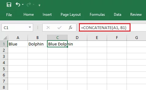
It works as demonstrated in the screenshot below:

 

 

The & and Concatenate Function in Excel

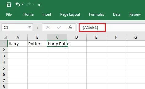
The concatenate Excel function works more or less the same as the ‘&’ or Ampersand function.

It acts like a substitute for concatenation in Excel and comes in handy since it is relatively quicker and easier to input.

The ‘&’ function lets you combine data in cells without using a complex function.

You can use the ‘&’ function to join together text strings or other data values, and resultantly, you would have the data of two cells combined in one cell.

The ‘&’ operation is used as explained in the screenshot below:

 

 

As seen, the ‘&’ function does the same work as concatenate function but is slightly more efficient to use. And the only thing that differentiates between these two functions is the limitation of strings.

Concatenation in Excel only allows input of values up to 255 strings, whereas the ‘&’ function does not impose any maximum limit.

But then again, people in daily life hardly ever need to combine a string as long as 255.

So the limitation of concatenate doesn’t have much influence, and the difference then comes down to the ease, efficiency, and comfort of use. You can choose whichever function suits you best.

For more on Excel, read our guide on Forecasts in Excel here.

 

Rules of Using the Concatenate Function

Although the Concatenate formula in Excel is simple and easy to apply, it does need a set of rules to work with; otherwise, it shows an error instead of returning values. The rules are listed as:

• When specifying a character or digit, arguments are a must, or the concatenate function will show the ‘#NAME?’ error instead of the output value.
• You can merge up to 255 strings or 1,892 characters in a single concatenate formula.
• Even if a single argument in the concatenate formula is wrong, the result would be a #VALUE error.
• You need to input at least one ‘text’ argument for the concatenate function to process and return value.
• The concatenation Excel function always returns value as a text string even if numbers are being combined.
• Excel concatenate function uses individual cell references since it doesn’t recognize arrays. This means you will have to write =concatenate(C4, C5, C6) instead of =concatenate(C4:C6).
• You don’t need to add quotation marks with numbers in the concatenate formula.
• The concatenate function allows a maximum of 30 arguments only in a single formula.

 

Using Concatenate

We know the syntax and basic requirements of the concatenate function. Let’s see how it works through a simple demonstration below:

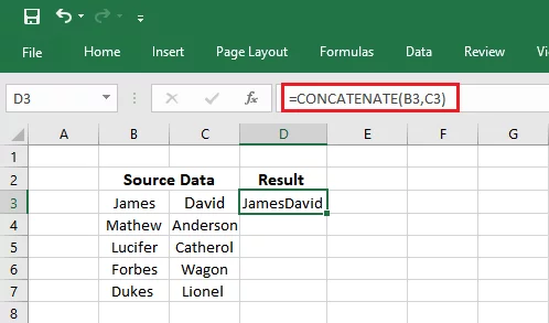
Consider two columns, B and C having certain values.

 

 

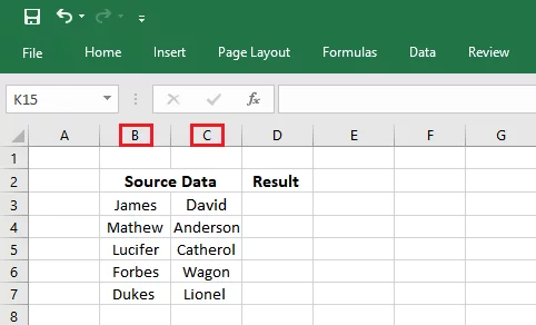
We use the concatenate function to combine the data in the first two cells.

We apply its formula using =concatenate(B3, C3) as shown in the image below.

 

 

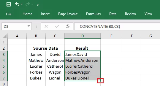
To copy the formula to the rest of the cells, simply drag the fill handle (the small green icon at the right bottom of selected cells) till the last value, as demonstrated:

 

 

That should clear the how to concatenate in Excel question in your mind. Also, if you want to delineate on your data set better, try adding borders to it. Read about adding borders to your worksheet in excel here. Let’s see some more examples further below.

 

Advanced Uses of the Concatenate Function

So far, we have discussed the primary usage of concatenate in Excel, but its applications don’t end here. While calculating data in Excel, we often need to combine values containing slightly different values than the usual formula.

These include commas, spaces, line breaks, hyphens or ranges, etc. To review these additional arguments, read on.

 

Concatenating Ranges  

Combining data from several cells at once is time taking and difficult. That’s because the concatenate function in Excel does not allow the usage of arrays, and in every argument, each cell needs to be referenced individually.

If you only have a small range to concatenate, for instance, from B1 to B5, you can enter each cell reference separately using the formula as below:

 

 

The task is easy with a small number of cells, but if you need to concatenate an extensive range, inputting each reference by hand might not be an option. So to ease you with that, we have jotted down three methods to help concatenate large ranges. These are as follows:

 

1. Use CTRL key to Select Multiple Cells

To select several cells simultaneously, simply press the CTRL key and select each cell you need to input in the concatenate formula. You can use the CTRL option as:

• • Input values in different cells.
  • Type the formula and its arguments in a new cell.
  • Press the CTRL key and release it only when every value you need has been selected.
  • Once released, add in the closing parentheses of the formula and press enter.

 

2. Merge the Cells

The easiest and quickest method to concatenate ranges in Excel is to merge them using the Merge across function under the Home tab. Before you combine fields using the Merge function, make sure you turn off the ‘merge all areas in selection’ option to select data in all cells. Next, click OK and that’s it. Your cells have been combined.

3. The Transpose Function

To concatenate a large range having more than 100 cells, we use the Transpose function as other methods might be slow to process such an extensive range. The result of the Transpose function is an array that is then replaced with separate cell references. If you’re unsure how cell references work, read our guide on Cell References here. The Transpose function is used as:

• • Select the cell where you want the concatenate function to return value and input the cell references for the Transpose function, say,

 

• • Press the F9 key in the formula bar with the cells already selected to change the arguments to calculated values. The formula will then show a number array.
  • Remove the braces from both ends of the formula.
  • Add =concatenate before the formula and enter the opening and closing parenthesis.
  • Once done, press the Enter key.

One thing to bear in mind is that no matter which method you opt for, the result value will be left-aligned, showing that it’s a text string even though each value might be a digit. That is because irrespective of the data entered, concatenate function always only returns a text string.

 

Inserting Spaces & Commas

Excel does exactly what it is told to, that means it won’t add spaces, commas or any other arguments unless fed into the input.

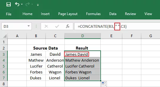
Say you want to add a single space between your text strings. You will need to add a space argument enclosed in double quotes like this “ “. Make sure you insert commas after and before each argument; otherwise, the formula will return an error instead of the expected value.

So the formula then becomes =concatenate(B3, “ “,C3)

The image below shows the use of arguments in the concatenation Excel formula.

 

 

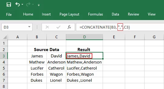
The same rule applies when you enter a comma during concatenation of two cells, the formula changes to =concatenate(B3, “,”, C3), and the string values would then be separated by commas as shown in the image below.

 

 

Including Line Breaks

For regular uses, we use delimiters to separate two text strings. But often, especially when combining mailing addresses, we use line breaks instead of adding punctuation marks, spaces or hyphens, etc.; for the Mac system, you would use carriage return and Windows uses line feed.

As explained before, the concatenate function does not add characters until it is asked to. So, to add a line break, you need to input a special function called ‘CHAR’ in the concatenate formula in Excel that provides the corresponding ASCII codes. The ASCII code for Windows Line Feed is CHAR 10, whereas, for MAC, the code for Carriage Return is CHAR 13.

Let’s understand the usage of line break with an example below. Say we want to post a mailing address, and all the data, postal code, city name, etc., are in different columns. We concatenate the values using the Ampersand function and input delimiters, including spaces, commas, and the CHAR 10.

 

 

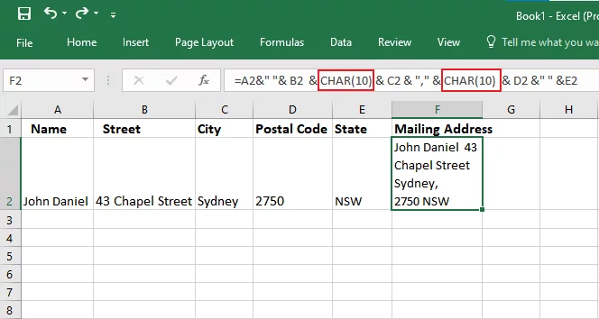
Once you input the data, type the formula, add the CHAR 10 and & function. In the image above, cell F2 shows the resultant value of the concatenate formula. Also, as the formula returns the value, turn on the Wrap Text feature so that the result is easy to read.

You can use ASCII codes for delimiters as well, but the easier way to use them is as applied in the example.

 

Working With Dates

We often need to concatenate digits or dates with a text string. When you combine two characters of different nature, you would want the nature of your result to be of your choice. And fortunately, Excel’s concatenate function provides you with this very facility by offering the TEXT function.

The TEXT function enables you to change the nature of the number by formatting it using format codes as per the need of your data. It is useful when you want to type a digit in numbers or combine values of two cells. Its syntax is as:

 

 

The standard font Excel offers is often not the first choice of people. To know how to format your font in Excel sheet, click here.

The syntax of the TEXT function consists of two arguments explained as follows:

• Value: Refers to the number that has to be concatenated with the text string. You can even use a cell reference.
• Format_text: Refers to a text string that specifies the style of the numeric value. The formatting is done using format codes.

To ensure your applied formula returns a value in the desired format, you need to use the TEXT function. In other cases, your result might seem broken or out of place. Let’s see an example below to better grasp the concept.

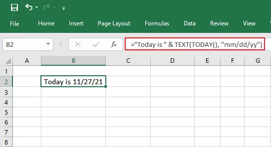
You can use either the concatenate function or the Ampersand function. We need to input date in cell B2 so the formula would be =”Today is” & TEXT(TODAY(), “mm/dd/yy”) as shown in the image below.

 

 

The TEXT function entered in this formula specifies the type of numeric value (here, the value was in date format) to be combined with the text string.

 

Troubleshooting: Why the Concatenate Function returns #VALUE!

The primary reason why you might be encountering the #VALUE! error could be an invalid argument in the concatenate formula, i.e., inputting a function in place of the parameter. If the answer of that function is an error, the concatenate function will return a #VALUE! error.

To avoid this error you can use the IFERROR function in the argument. It would check each cell in the formula for #VALUE error and if issue exists, it would omit that particular cell and return value from the rest of the cells. The formula is written as:

 

 

The #VALUE error may also appear if the formula includes empty cells. You can rectify the issue under Tools tab in Formatting Auditing group by selecting Evaluate Formula.

 

Reverse of Concatenate

Reversing the concatenate formula means splitting the data you combined into one cell into two or more cells. The reverse does the complete opposite of what the concatenate formula is used for. There are two basic ways to reverse the concatenate function. These are as follows:

• Using Formula
• Using Text to Columns

 

Using Formula

The formula used to reverse the concatenate function might seem complicated but is utterly simple when used. It uses the Trim, Mid, Substitute, Rept. and Columns formula to split the values. Say, you have values in cells C2-C5 and you need to put them in different columns, you use the formula as:

 

 

Apply the formula in a new cell, and it will look something like the formula in this image.

 

 

Once the formula has been entered and the return value is correct, simply drag the fill handle down to the cell you want your values. It is demonstrated in the image as below:

 

 

One thing to bear in mind here is that even if you select more cells than the values entered, the formula will not show any error, and the extra cells will be left empty.

 

Using Text to Columns

Like using formulas, using Text to Columns will help you reverse the concatenate function. This method uses a number of steps which are discussed below:

• Whether manually or using some technique, select each cell in which you want to reverse the function.

 

 

• Next, open the Data tab, and under the group of data tools, select the Text to Column command.

 

 

• A Convert Text to Column Wizard Dialog Box appears on the screen. Under Original Data Type, select Delimited and press Next.

 

 

• Check the Other option and type in whatever delimiter you want to use.

 

 

• In the next dialog box, choose General and select the location where you want the reverse of concatenate to be displayed. Once done, press the Finish button.

 

 

• The return value should look something like this:

 

 

Difference Between Concatenate and Other Functions

Almost all of the functions used to combine values in Excel work the same and give similar results. However, there might be a tad bit of difference in their arguments, application, and requirements. Some functions that work the same as Concatenate function in Excel are described as below:

 

Concatenate VS. Concat

The Concat function is primarily a new version of the Concatenate function and has replaced it in all successive versions of Microsoft Excel after the 2016 version. It functions the same as the Concatenate function with an advanced feature to concatenate a range of cells having text strings, i.e., =concat(B1:E5).

This very feature was not present in the Concatenate function, and you would need to do the task manually but now you have an option. The best part about Concat is that it ignores blank cells, unlike the concatenate function. That means you don’t have to worry about the empty cells included in the formula.

The Concatenate function is although available in the latest version of Excel; there is a high chance Microsoft might disable it in the versions to come.

 

Concatenate VS. Merge

Concatenate function combines the data from two different cells into one new cell. On the other hand, Merge is used to physically merge two cells into one single cell, irrespective of the values in the cell.

Merge function is better to use when you need to input data in various columns under a single cell heading, and concatenate is used when you need to put together values of two cells into one cell. The Merge function was introduced in the older versions of Excel 2007-2008 and is still being improved.

 

Concatenate VS. Textjoin

The Textjoin function is used to join strings or ranges with the assistance of a delimiter. The function uses a minimum of three arguments. Whereas Concatenate function mainly deals with values in cells only and not ranges.

The best thing about Textjoin is that it lets forego empty cells. It is mainly used when you need to concatenate an array with a desired delimiter. Concatenate, on the other hand, simply combines values. The Textjoin function was introduced in the older version of Excel 2016.

 

Final Verdict

When the need to combine a huge number of cells arises, the Concatenate function is your silver bullet. While some users find the Concatenate function of excel outdated, it is undoubtedly a quick way to put together values that are otherwise difficult to manage. Using concatenate in excel is easy and all you need is some practice to become the next Concatenate Expert.

But to make anything work, the input has to be correct. So make sure you enter the correct formula, proper arguments and suitable values. That brings us to the end of our post. Happy Excel Working!