
Using A Data Table To Create A Pivot Table [Quick & Easy!]
Have you ever considered turning your list into a Data Table?
From this, you can easily create a Pivot Table.
A Pivot Table is a table of values which are aggregations of groups of individual values, much like a histogram!
This would be beneficial if your data source was constantly changing, as you’ll see!
Pivot Tables are covered on the advanced Excel course in London that we run monthly.
Using an Excel List
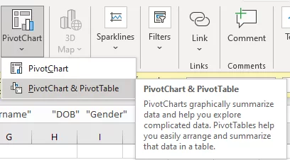
Start by going to the insert tab and hit the Pivot Chart button.
Then in the drop-down menu, click PivotChart & PivotTable.
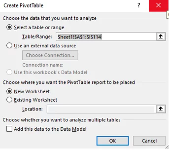
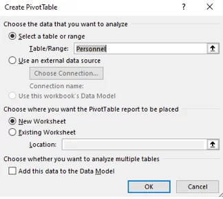
When creating a Pivot Table, you specify the Table/Range, or just any rows or columns you need for that Pivot Table, then click OK.
As below in the dialog box, A1-I114.
If at a later point, the source data has more rows/cols added to it, the Pivot table will not pick up the new data.
Refresh will also not help as this can only be used to update if the original data has changed, such as a salary, so the data range would have to be updated.
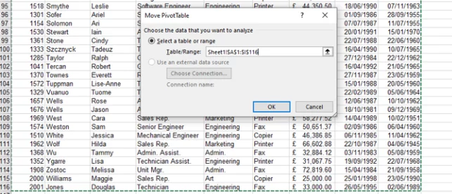
You can do this by clicking in the Pivot Table and choosing the Analyse Menu and Change Data Source.
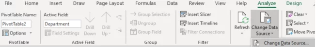
This would place you back on the original data, enabling you to select the new range for the Pivot Table in the dialog box.
However, if you convert your original data range into a data table, you only need to refresh as new data is added.
This is because a data table will have a name applied to it, you can also change this name if you wish.
Setting up the Data Table
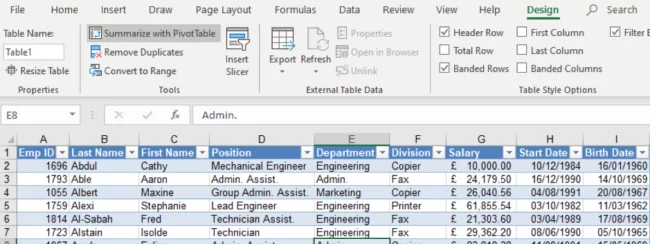
Click in your Excel List and, from the HOME Ribbon, choose FORMAT AS TABLE.
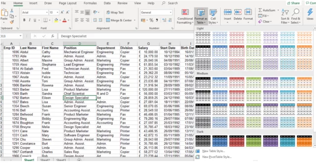
Here you can choose the Colour Scheme for your table.
If you combine this with different font formatting, you will get much better looking tables!
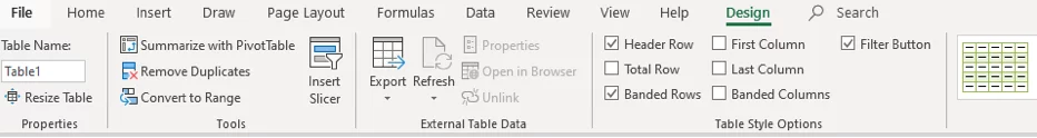
Once the Excel table has been created, notice that a new ribbon (Toolbar) appears in your Menu Tabs – DESIGN.
If you click outside the data table, this will disappear, so make sure you are within the data table to use the Design Menu.
If the values area looks incorrect, this is because sometimes Excel has analysed your data incorrectly.
You can change the way the Pivot Table is calculating values by clicking on the arrow to the right of the field name, then selecting the Value Field Settings.
From here, simply change the calculation in the Summarize Values By section, and your Pivot Table data should correct.
The Table will have been named for you in this instance Table 2, shown on the left-hand side of the ribbon.
This name can be changed, all you have to do is highlight the name in the Table Name box and overtype it.
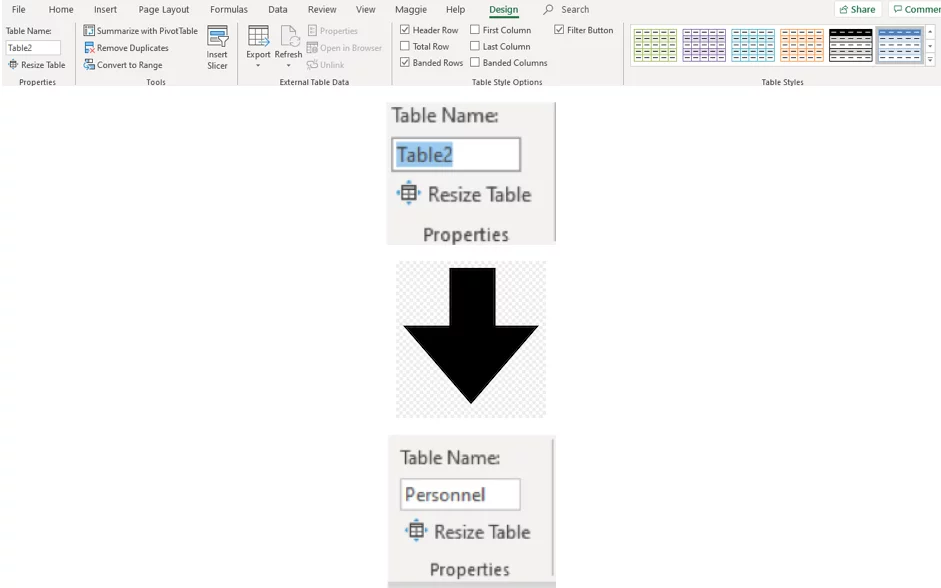
The name will apply to the entire data in the list.
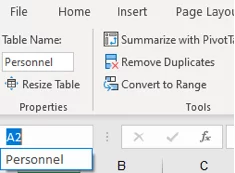
If you select the Name box you will see the name in here, if you click on this it will highlight the entire range.
As extra data is added to the data table, the name will automatically extend to include these new rows/columns.
The same if rows/columns are deleted.
Creating The Pivot Table
Now that the Data Table has been created, we can create a Pivot Table can from the Design Ribbon.
Click in your data table, the Design Ribbon will appear and choose SUMMARIZE WITH PIVOT TABLE.
Notice that the Data Table name appears in the Create Pivot Table box, instead of the range.
As you adjust the rows and columns in the original list, include these in your pivot table and click ok.
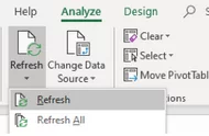
Tip: You can refresh a Pivot Table with a right click over the top of it, or by selecting the Analyse Menu and Refresh.
Using the second method, you can refresh all Pivot Tables built off the original data by selecting Refresh All.
Pivot Tables are very data-centric, making flowcharts from your data offers a more visual style of presentation.
Choosing the right way to present your data is very important, always think about the audience!
Final Thoughts
Overall, learning to create a Pivot Table from a Data table is a great tool.
The main reason for this is the fact that these Pivot Tables are appropriate when your data source is constantly changing.
Every Excel user can benefit from learning this skill.
Making a decision between what kind of Pivot Table you want to create is important!


- Facebook: https://www.facebook.com/profile.php?id=100066814899655
- X (Twitter): https://twitter.com/AcuityTraining
- LinkedIn: https://www.linkedin.com/company/acuity-training/