TRIMRANGE Function In Excel

The TRIMRANGE function in Excel is used to automatically remove blank rows, columns, or both from a specified range.

It’s especially useful for cleaning up data before feeding it into formulas, charts, pivot tables, or dropdown lists.

TRIMRANGE helps ensure that your data ranges are clean and compact, which prevents errors and improves performance when working with dynamic reports or automated workflows.

Common uses include:

• Cleaning up raw data imports from external systems
• Preparing dynamic ranges for use in charts or validation lists
• Removing excess blank space before passing data into other formulas like FILTER, SORT, or UNIQUE

Want to sharpen your Excel skills? Check out our full range of Excel Courses to level up fast.

Basic Syntax

=TRIMRANGE(range, [ignore_blanks], [trim_direction])

Here’s What Each Argument Means:

• range – The cell range you want to clean. This is the only required argument.
• ignore_blanks (optional) – Set to TRUE to ignore visually blank cells that contain formulas like =””. If omitted, Excel defaults to treating those as non-blank.
• trim_direction (optional) – Controls whether to remove rows, columns, or both. Common values include:
  • “rows” – removes blank rows only
  • “columns” – removes blank columns only
  • “both” – removes both blank rows and columns

Note: Depending on your Excel setup, TRIMRANGE may be part of a custom function library, VBA module, or Power Query script.

If it’s not recognized by default, it may require enabling add-ins or using a dynamic array-enabled version of Excel.

How TRIMRANGE Works

TRIMRANGE scans the specified range and removes all blank rows, columns, or both depending on the direction you set. The result is a cleaner, resized range without extra empty space.

This is especially helpful when you’re:

• Feeding clean data into pivot tables, charts, or dropdowns
• Automating dynamic reports
• Working with data that frequently changes in shape or size

By trimming away the blank areas, TRIMRANGE makes your spreadsheets more efficient and easier to maintain.

What Is A Dynamic Range?

A dynamic range is a cell range that automatically adjusts in size as your data changes.

Instead of referencing a static range like A1:C10, dynamic ranges grow or shrink based on the actual content in the sheet.

This is incredibly useful in formulas, charts, pivot tables, and dashboards where the underlying data isn’t always a fixed size.

Dynamic ranges can be created using tools like:

• Excel Tables – Expand automatically as you add new rows.
• Spill formulas – Like =SORT(A1:A100), which dynamically fills adjacent cells.
• Named ranges with OFFSET or INDEX – More complex but fully customizable.

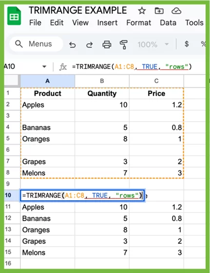
Simple Example

Let’s say you have a table of sales data where some rows are blank.

Formula:

=TRIMRANGE(A1:C10, TRUE, “rows”)

This removes any entirely blank rows from the range.

Result: A smaller, clean table with only the active data rows remaining.

Complex Examples

Let’s explore how TRIMRANGE can solve more advanced, real-world problems – especially when working with dynamic datasets that include a mix of formulas, user input, and blanks.

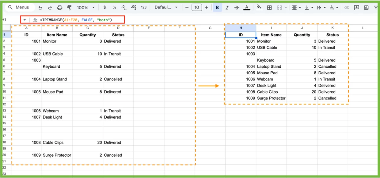
Example 1: Cleaning Messy Imported Data

You’ve imported sales data from a database export that includes both blank rows and empty columns. You want to clean the dataset before using it in charts or pivot tables.

Formula:

=TRIMRANGE(A1:F20, FALSE, “both”)

This removes all empty rows and columns, leaving only the structured part of the dataset.

Example 2: Nesting TRIMRANGE With AVERAGE

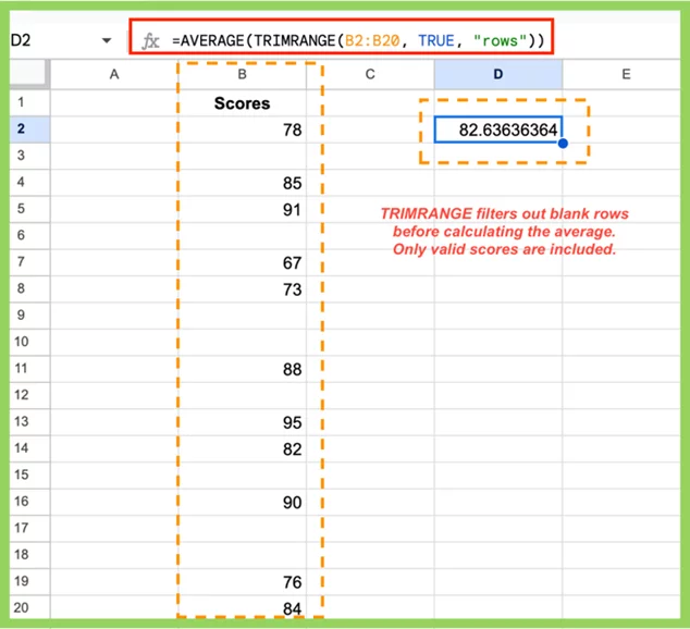
Now, suppose you have a column of numeric scores in B2:B100, with some rows blank. You want to calculate the average only for the populated values, without having to manually clean the data.

Formula:

=AVERAGE(TRIMRANGE(B2:B100, TRUE, “rows”))

Here, TRIMRANGE feeds only the valid values into the AVERAGE function, preventing errors or skewed results caused by empty cells or formula blanks.

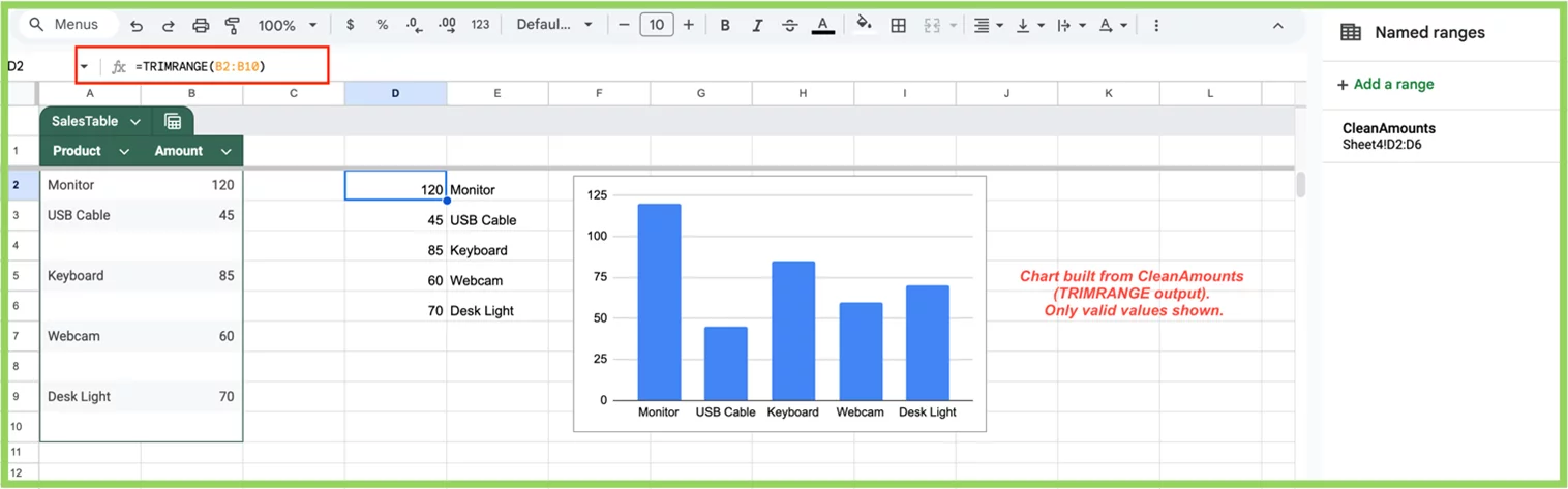
Example 3: Dynamic Named Range Cleanup for Charts

You’re building a live dashboard where users update entries in an Excel Table. However, your chart still includes blank entries when users clear old data.

To fix this, you create a dynamic named range with TRIMRANGE, then feed that into your chart:

Named Range Formula:

=TRIMRANGE(SalesTable[Amount], TRUE, “rows”)

Then assign that named range as the chart source. This ensures the chart always reflects only populated values, without displaying blank points.

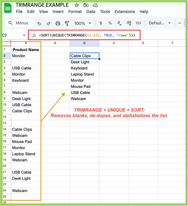
Example 4: Combining With UNIQUE and SORT

You have a long list of product names (some blank, some duplicated), and want to:

1. Remove blanks
2. Remove duplicates
3. Alphabetize the result

All in one go.

Formula:

=SORT(UNIQUE(TRIMRANGE(A2:A100, TRUE, “rows”)))

This combination creates a clean, sorted dropdown list, perfect for validation rules or slicers.

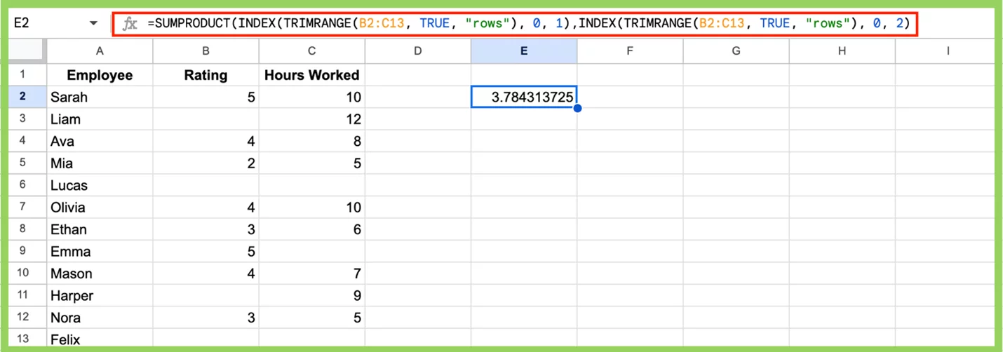
Example 5: Calculating Weighted Average on Filtered Data

Imagine you’re tracking staff performance, but some rows are incomplete or contain blanks. You want to calculate a weighted average rating, but only using rows with complete data.

Assume:

• Column A = Employee Name
• Column B = Rating (1-5)
• Column C = Weight (e.g., project hours)

Some employees have only a rating or only logged hours, but you want to include only the rows where both values are present, to avoid mismatches or padding errors.

To do this, you can use the following formula:

=SUMPRODUCT(INDEX(TRIMRANGE(B2:C13, TRUE, “rows”), 0, 1), INDEX(TRIMRANGE(B2:C13, TRUE, “rows”), 0, 2))/SUM(INDEX(TRIMRANGE(B2:C13, TRUE, “rows”), 0, 2))

This formula works by first using TRIMRANGE to clean the dataset, it removes any row where either the rating or hours column is blank.

Then, the INDEX(…, 0, 1) extracts the cleaned ratings, and INDEX(…, 0, 2) extracts the cleaned hours worked.

The SUMPRODUCT multiplies each rating by the number of hours, and divides by the total hours to produce the correct weighted average.

In our example, the result is 3.78, calculated from only the rows with complete data.

Why This Matters

In dynamic spreadsheets, data shapes constantly change. Rows get added, deleted, or partially filled. TRIMRANGE ensures your formulas, charts, and reports only act on clean, usable data.

Combined with other Excel functions, TRIMRANGE enables robust, automated workflows without relying on helper columns or manual cleanup.

Troubleshooting TRIMRANGE

Here are some common issues and how to fix them:

1. #REF! Or #VALUE! Errors
   • Make sure the range is valid and not returning a completely blank result.
   • Double-check formula syntax.
2. Function Not Recognized
   • TRIMRANGE may be part of a custom add-in or dynamic array lab feature.
   • Check that your Excel version supports it or if it requires enabling via VBA or third-party tools.
3. Structured Tables Behaving Oddly
   • If you’re referencing Excel Tables, TRIMRANGE may not behave predictably.
   • Consider converting the table to a standard range.
4. Preventing Errors

Wrap TRIMRANGE in IFERROR() to avoid user-facing problems:

=IFERROR(TRIMRANGE(A1:C20, TRUE, “rows”), “”)

Conclusion

The TRIMRANGE function is a powerful asset for anyone working with dynamic or messy datasets. It allows you to:

• Quickly remove blank rows or columns
• Clean up data before feeding it into charts, dropdowns, or pivot tables
• Combine with other functions to build automated, dynamic solutions

Whether you’re building dashboards, validating inputs, or preparing reports, TRIMRANGE helps you keep your data streamlined and reliable.

Start small, test your formulas, then explore combinations with AVERAGE, VLOOKUP, or FILTER for more advanced workflows.