
The Ultimate Guide To Excel Drop Down Lists
Contents
What if the key to collaborating in Excel was a different way of making tables?
We have all used tables in Excel, but what if you are looking to make this table into a list for others to use?
You can easily allow users to choose an item from a pre-defined list, by using a dropdown list in Excel.
When you are creating a dropdown list, Excel allows you to tailor it to your needs in a variety of ways.
Why Use A Drop Down List?
These types of lists are great for user input.
It’s a great way to ensure that only valid data is entered into a cell.
Drop down lists help you to organise your data and limit the amount of entries people can make to each cell.
Whenever you create an Excel spreadsheet for a user to input data, a drop down list will be very helpful!
They help you to streamline the experience you are creating for your users, and design a smooth looking document for them to use.
Creating a clear and simple workbook is a very valuable skill to employers, always covered on our Microsoft Excel courses near Liverpool Street.
We will cover everything about how you can make a drop down list here.
Drop Down List – Cell Range
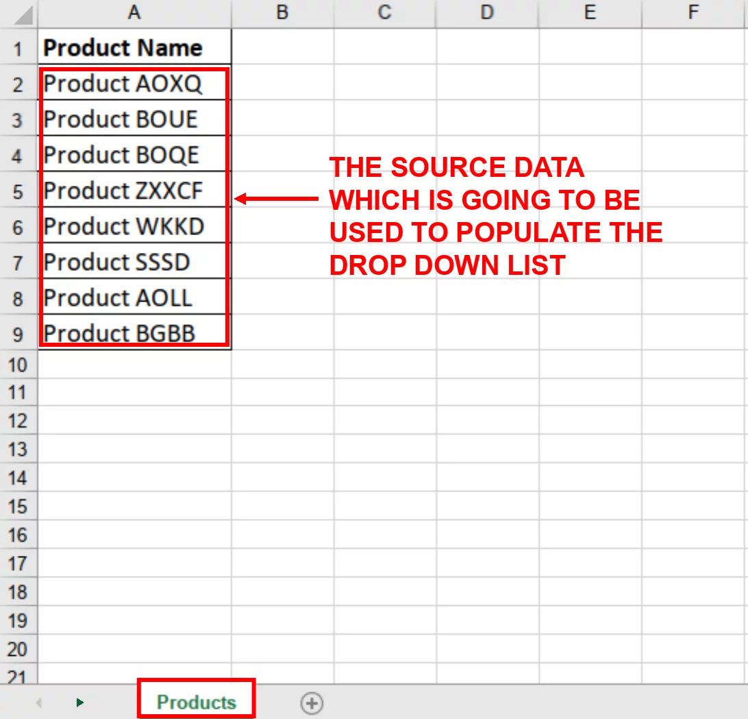
In the example below, we have a worksheet called Products containing the names of products.
This is the original sheet that contains the source data.
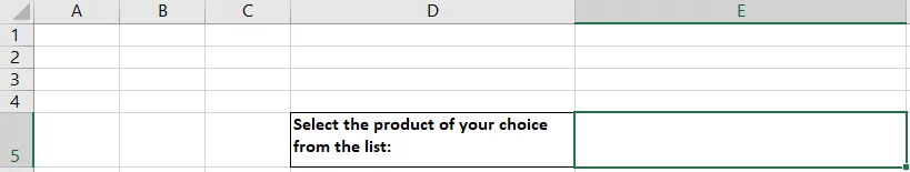
1. Now select or create another sheet. In this case, this is the destination sheet where you would like the drop down list to be.
This sheet is called ProductsDropDownList in our example.
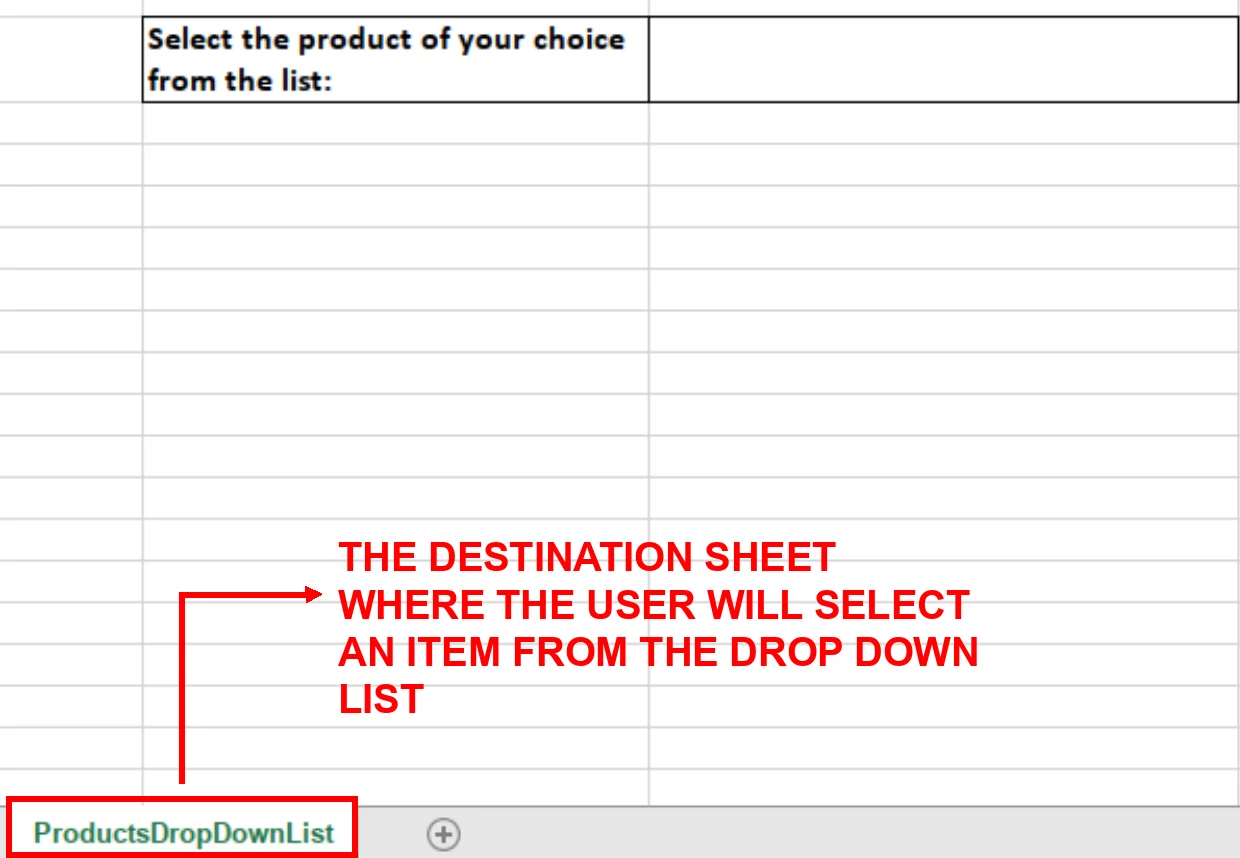
2. Select cell E5 on the destination sheet. This is the cell that is going to have the drop down list.
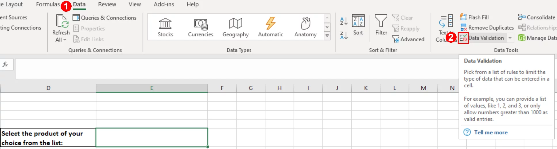
Go to the Data Tab on the ribbon and on the Data Tools group, choose Data Validation.
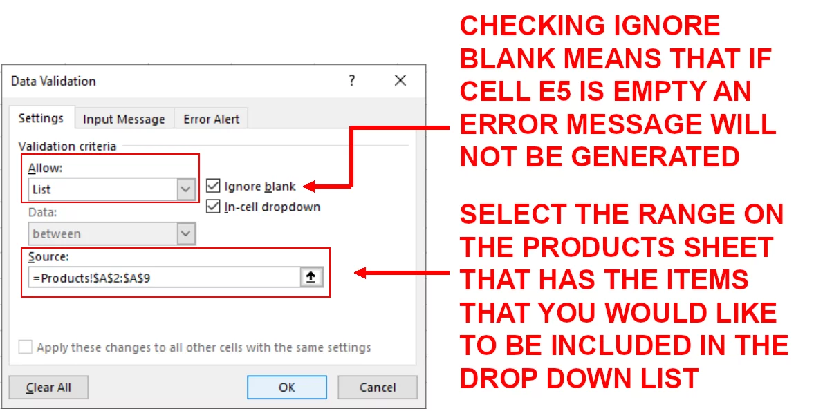
3. The Data Validation Dialog Box will appear. Under the Settings tab, in the Allow drop down menu click List.
Ensure Ignore blank and In-cell dropdown are checked.
Using the Source box, select the cell range on the Products sheet, which in this case is range A2:A9.
4. Click Ok.
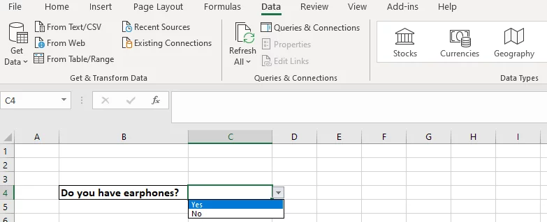
5. The drop down list is shown below.
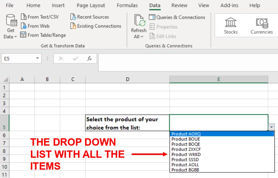
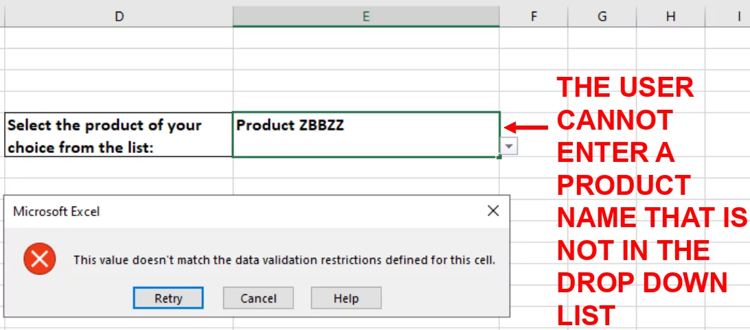
If the user tries to type a value in the cell that is not in the drop down list, they will get an error message.
• Note: The drop down box arrow in Excel is only shown when the cell containing the drop down list is selected.
With all the cells selected decrease the font size by one point. Then increase the zoom level magnification.
In the example below 140% zoom level magnification was used and the items in the dropdown list now look bigger.
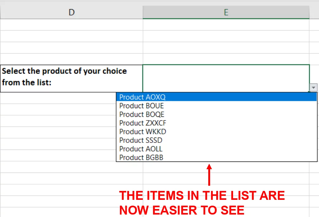
You can keep it like this by using font formatting to change the size of the text, regardless of the zoom.
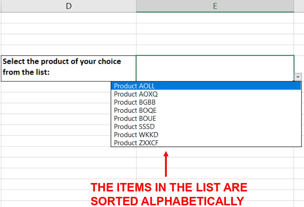
• Tip: By default, the items in the list will appear in the same order that they are entered in the original worksheet.
If you’d like to have the items in your list sorted in either ascending or descending order, go to your source data.
Then with one cell in the range selected, go to the Data Tab:
In the Sort & Filter group choose either ascending sort or descending sort.
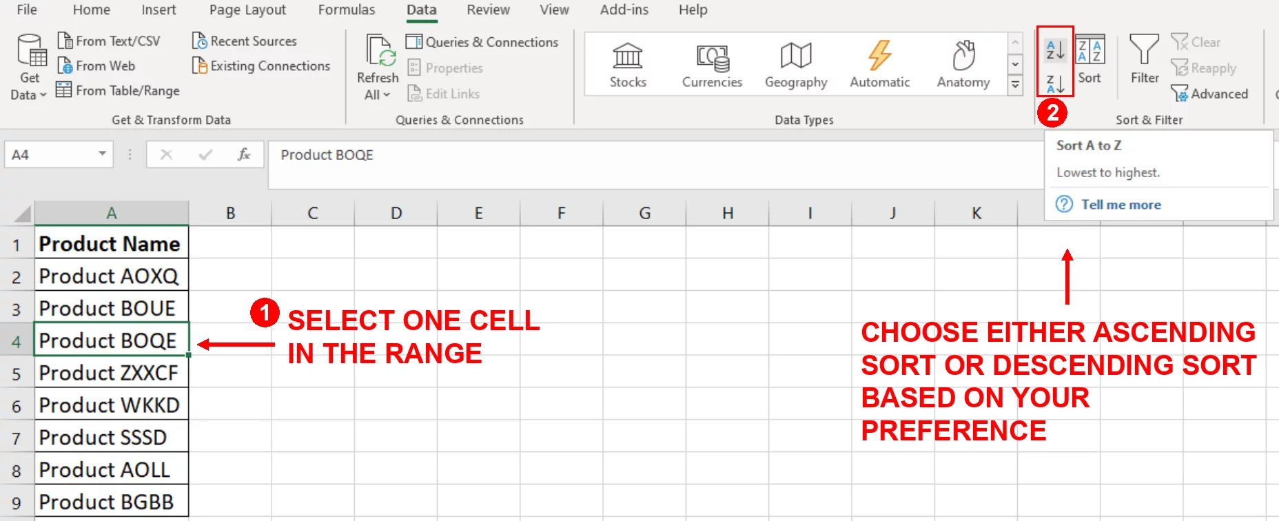
In the example below, ascending sort was selected. The items in the drop down list are now sorted in alphabetical order.
• Tip: You can hide, or password protect the worksheet that contains the source data!
This is great if you don’t want people to accidentally edit or remove items in your dropdown list.
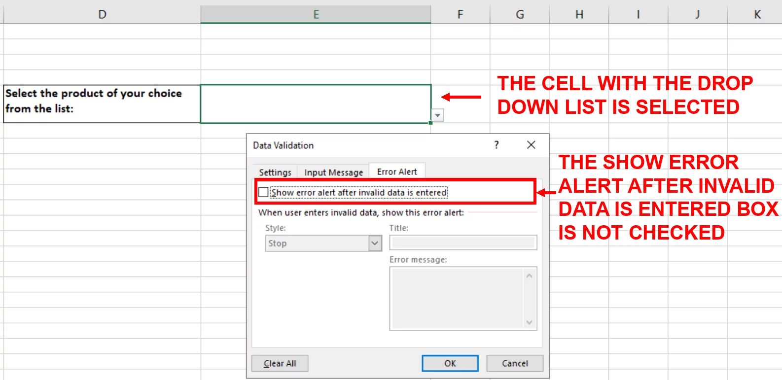
You can also allow the user to enter another item that is not in the list, when necessary.
To do this select the cell containing the drop down list.
Go to the Data Tab on the ribbon and on the Data Tools group, choose Data Validation and navigate to the Error Alert Tab.
In the Error Alert Tab: uncheck the check box that says Show error alert after invalid data is entered. Click Ok.
Add An Item To A Drop Down List
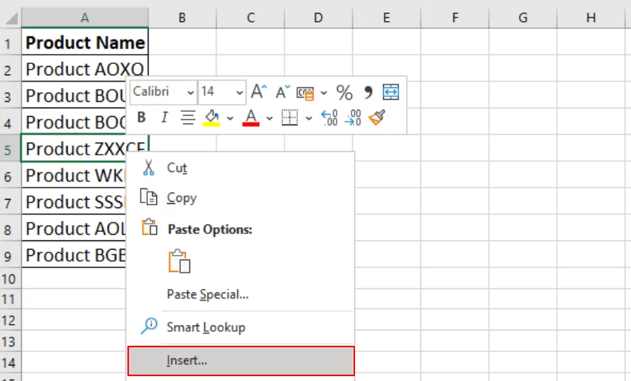
You may have a situation where you want to add a product that is not in the original list.
1. To do this, go to the original sheet containing the names of the products. Select one of the products.
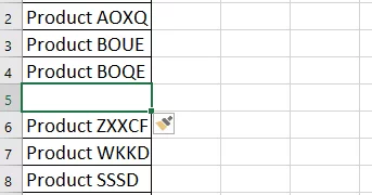
2. Right-click the cell and select Insert.
3. Select the Shift cells down option. Click Ok.
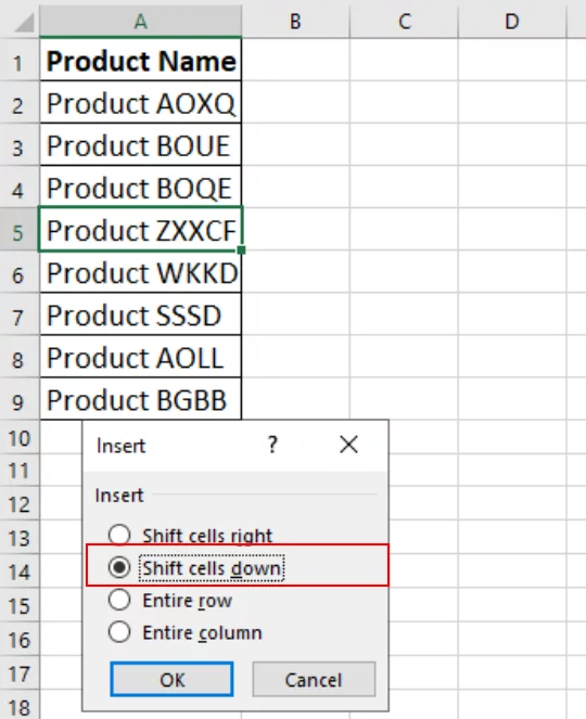
Once you have done this you will see the the following.
4. Enter a new product name.
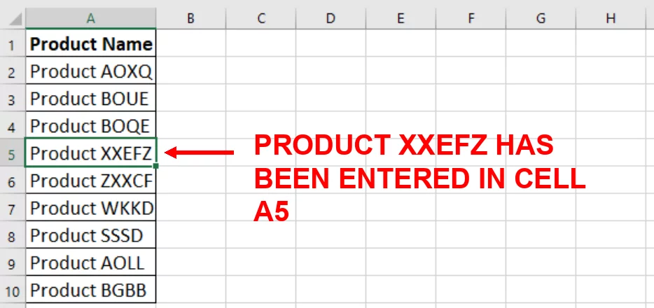
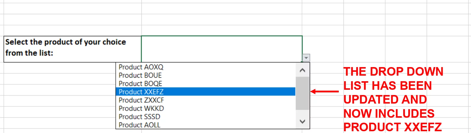
5. Now when you return to your sheet with your drop down menu, you should see the list has been updated.
Delete An Item – Drop Down Lists
You may have a situation where you want to delete a product from the drop down menu, such as when you find an outlier in your data you want to omit.
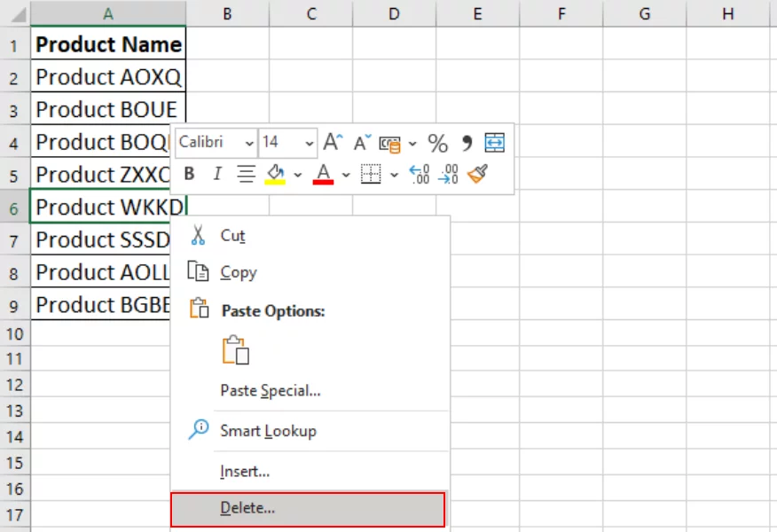
1. To do this, go to the original sheet containing the names of the products.
Select the item that you want to be deleted from your drop down menu.
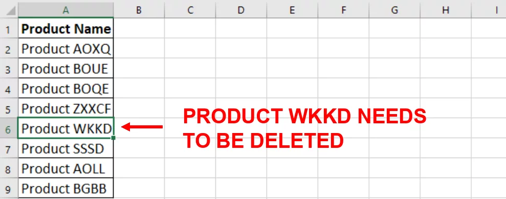
2. Right-click the cell and select Delete.
3. Select the Shift cells up option. Click Ok.
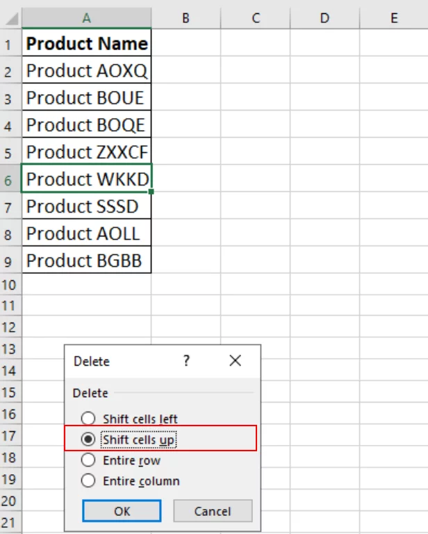
Once you have done this you will see the the following.
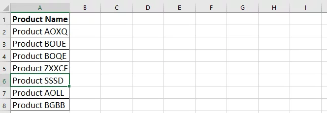
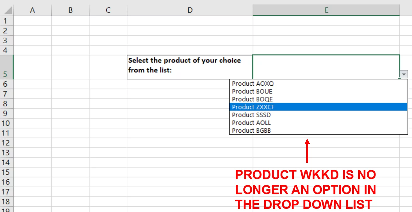
4. This item should no longer be in the drop down menu.
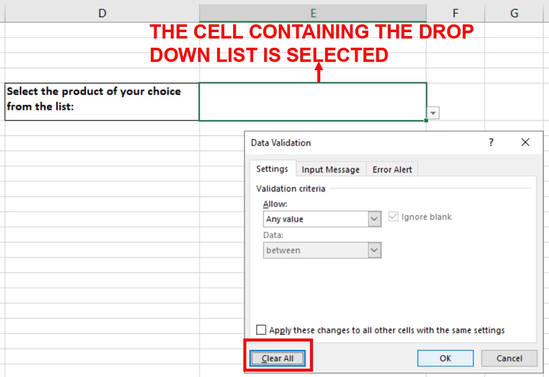
Remove A Drop Down List
For removing drop down menus, Microsoft Excel lets you do this in two main ways.
Select the cell with the drop down list.
Go to the Data Tab on the ribbon and from the Data Tools group, choose Data Validation.
Under the Settings tab, click Clear All and then OK.
The drop down list will be removed from the cell.
Once you have done this you will see the the following.
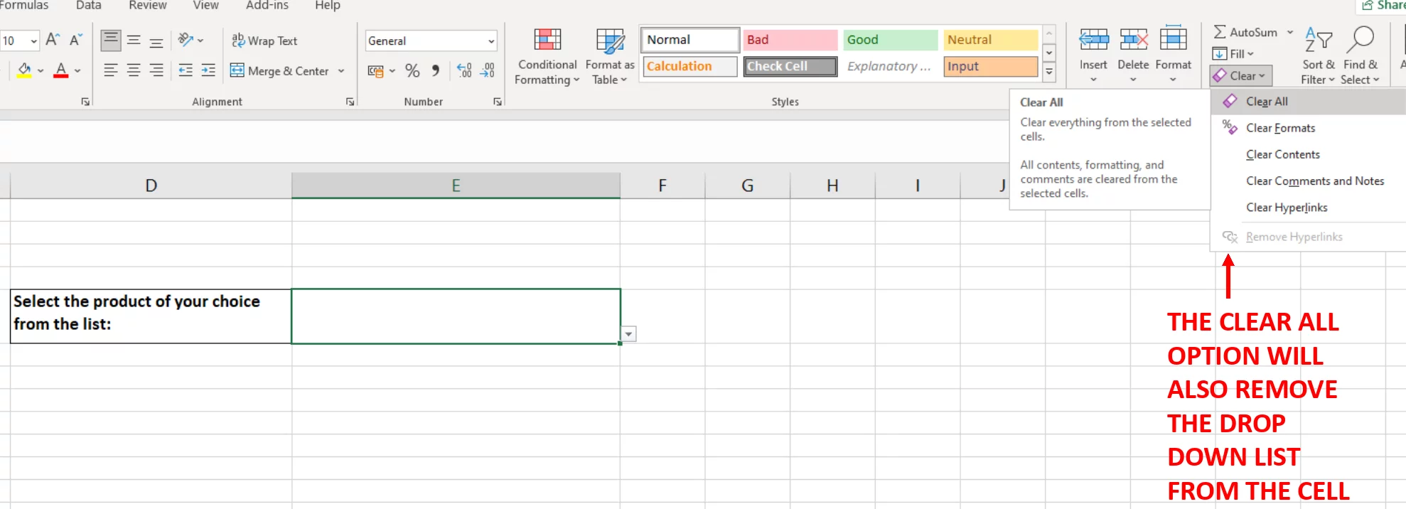
You can also remove the drop down list by selecting the drop down list and then going to the Editing group, and clicking clear all.
However if the problem is within the data you selected for the drop down list, you can instead remove a specific cell from the data.
Once you have done this you will see the following.
Drop Down List – Manual Data Entry
You can manually enter the source data for the drop down list by using the Source box.
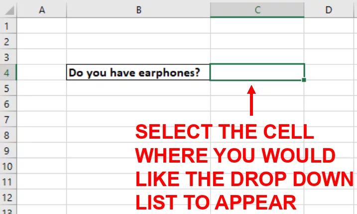
1. Select the cell which you would like to contain the drop down list.
2. Go to the Data Tab and choose Data Validation from the Data Tools group.
Select List and this time in the Source box manually type the entries as shown below.
Make sure that each entry is separated by a comma.
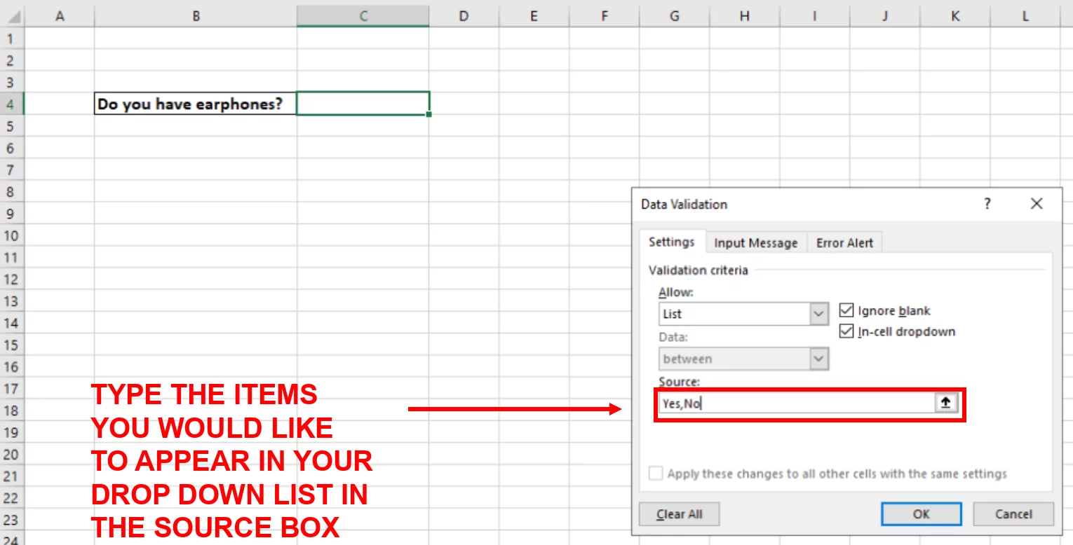
3. Click Ok.
Drop Down List – Named Range
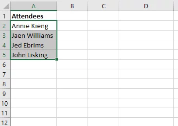
You can use a named range as your source for your drop down menu, which is a range of cells with a name assigned to help you identify it.
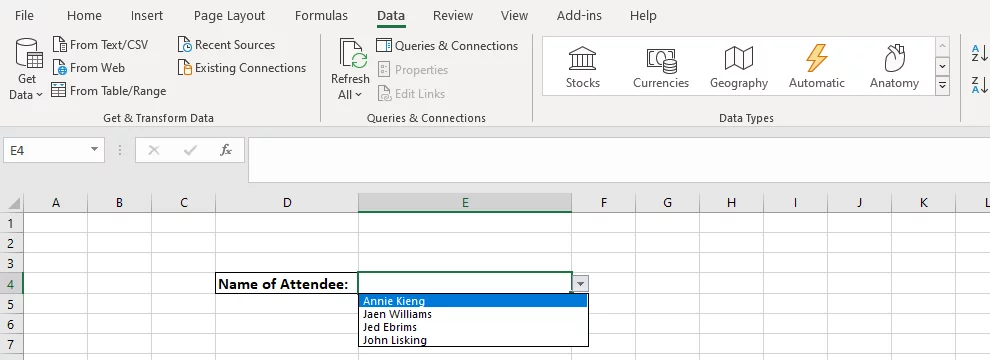
1. Create a named range first. Select the range of cells that you would like to name.
2. Type the name Attendees into the Name Box and press Enter.
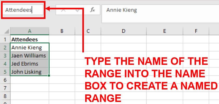
3. In the cell where you would like your drop down list to be, follow the same steps to create a simple drop down list.
But first, in the Source box type an equals sign first and then the name of your named range.
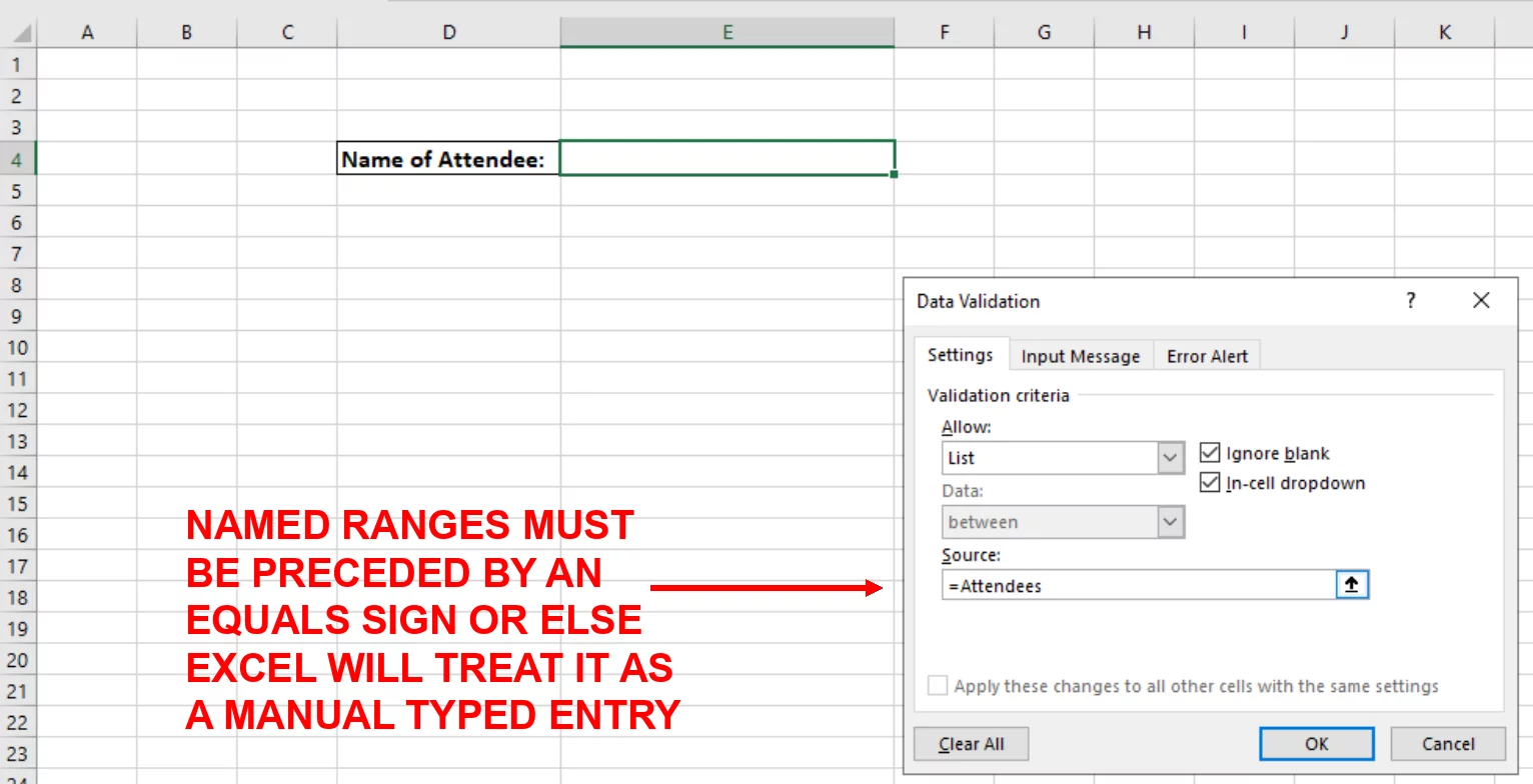
4. Click Ok.
Conclusion
Making a drop-down box in Excel is great for making your sheets and dashboards more appealing.
It will speed up your data entry and minimise the risk of errors effecting your work.
Always keep this technique in mind when thinking about collaborating!


- Facebook: https://www.facebook.com/profile.php?id=100066814899655
- X (Twitter): https://twitter.com/AcuityTraining
- LinkedIn: https://www.linkedin.com/company/acuity-training/