
News & Tips
AllAdobe InDesignAdobe PhotoshopManagementMicrosoft ExcelMicrosoft Power AutomateMicrosoft Power BIMicrosoft PowerPointMicrosoft ProjectMicrosoft SharePointMicrosoft WordPresentation SkillsSQLTime Management

Line Manager Skills – Progressing Your Career
Line management is more than just overseeing work. It’s about building trust, supporting people, and driving results. Whether you’re preparing for your first leadership role or already managing a team, line manager skills can transform both your performance and your…

How Presentation Skills Empower Your Career
Whether you’re presenting project results, pitching ideas, or just speaking up in meetings, presentation skills can dramatically boost your career. In this article, we’ll explore why presentation skills matter, how they improve your performance in your current role, and how…
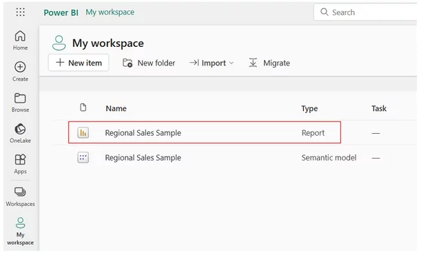
Using Publish to Web in Power BI
Power BI’s “Publish to Web” feature is a powerful tool for sharing interactive reports and dashboards with a wider audience. Whether you’re a data analyst, business owner, or educator, it enables you to embed live Power BI visuals in websites,…

Power BI Terms Explained: A Glossary for Beginners
Power BI has its own jargon and language. Whether you’re exploring a dashboard, chatting in a team, or diving into Power BI training, understanding key terms helps you make sense of it all – fast. Here’s your go-to guide! ⚙️ Common Power BI…
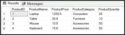
SQL Insert Multiple Rows
If you regularly need to add lots of new data to a SQL table, manually inserting each row can be slow and repetitive. One of SQL’s great strengths is it lets you insert multiple rows in one go. In this…
How To Start Learning Excel – Methods That Work
Microsoft Excel is still one of the most powerful and widely-used tools in the business world. Whether you’re managing budgets, analysing data, or organizing workflows, Excel can streamline and simplify your work. But getting to grips with all that it…

The WHERE Clause – SQL Master Guide
One of the most fundamental and powerful tools in SQL is the WHERE clause. It’s your primary way of filtering rows in a database query to return only the data that matters, and a fundamental part of our SQL training…

Power BI Turns 10: How It Changed Business Intelligence Forever
In July 2025, Power BI celebrates a decade of transforming how organizations work with data. What started as a bold move by Microsoft to bring business intelligence to the masses has grown into a globally recognized platform used by millions…

The Best Ways To Learn Power BI
Power BI is one of the most powerful tools for transforming raw data into interactive, insightful dashboards and reports. As more businesses seek data-driven decision-making, mastering Power BI has become an essential skill for analysts, business intelligence professionals, and even…
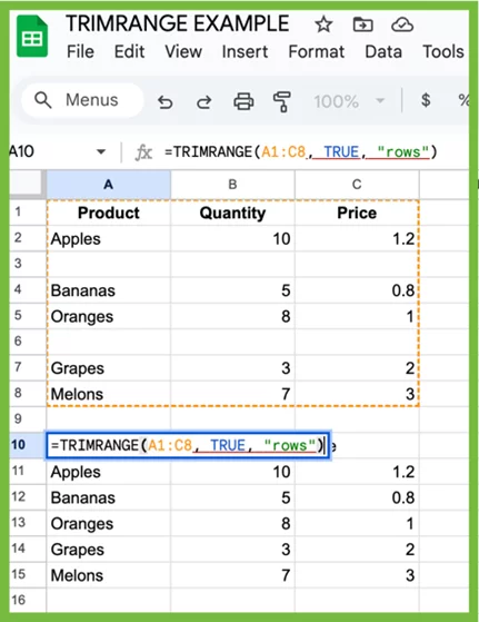
TRIMRANGE Function In Excel
The TRIMRANGE function in Excel is used to automatically remove blank rows, columns, or both from a specified range. It’s especially useful for cleaning up data before feeding it into formulas, charts, pivot tables, or dropdown lists. TRIMRANGE helps ensure…

Your Voice Is an Instrument – Are You Tuning It?
In the world of public speaking, your voice isn’t just a tool, it’s your primary instrument. Just as a musician wouldn’t perform with an untuned instrument, a speaker shouldn’t step in front of an audience without tuning their voice. Understanding…

The Confidence Loop: How Small Wins Lead to Bigger Stages
Confidence in management and public speaking isn’t born, it’s built. And it’s built through a process known as the confidence loop. Whether you’re giving your first team update or speaking on a main stage, every speaker starts the same way:…
- Facebook: https://www.facebook.com/profile.php?id=100066814899655
- X (Twitter): https://twitter.com/AcuityTraining
- LinkedIn: https://www.linkedin.com/company/acuity-training/