­Master The XLOOKUP Function In Excel!

It’s time we introduce you to the new member of the modern function family of Excel – the XLOOKUP function. XLOOKUP is the successor to the conventional VLOOKUP, INDEX & MATCH, LOOKUP, and the HLOOKUP function.

You must have heard the meme floating on the internet these days that says.

There are two types of people in the Excel world; the type that masters VLOOKUP & XLOOKUP. And the type that hovers about the ones who master VLOOKUP and XLOOKUP!

Which type are you? If you have been ‘type two’ all this time, this article is sure to pave your way to ‘type one’.

Don’t just stop here! – check out our wide variety of other Excel courses offered by Acuity training.

 

XLOOKUP Explained

VLOOKUP paired together with the INDEX & MATCH function that took a whole lot of science to accomplish an operation has now turned into a child’s play. Through the XLOOKUP function, Excel has offered a one-in-all solution to all the VLOOKUP problems of Excel users.

It allows you to look up data, both horizontally and vertically, to the above and the left. Users can define multiple criteria and can seek a whole row or column of data as the return value instead of a single value only.

This powerful successor of the VLOOKUP function is all that Excel users have been pleading for the last three decades.

But how can you learn all the above functionalities of the XLOOKUP function? Stay connected till the end to master them all.

 

Syntax

The syntax of the XLOOKUP function looks as below.

 

 

A little too long to decipher? Let’s break it down into individual arguments to make better sense of it.

 

Arguments

• • Lookup_Value – the first argument represents the value to look for in a given dataset.
  • Lookup_array – the second argument refers to the data range where the value is to be looked for.
  • Return_Array – the third argument refers to the array/range from where the value that is to be returned.
  • If_not_found – the fourth argument is an optional one that refers to the value to be returned if the desired value is not found. If the lookup value doesn’t exist in the data set and the ‘if_not_found’ argument is omitted, Excel returns the #N/A error.
  • Match_Mode – the fifth argument is also optional. It refers to the match type to be performed by Excel:

• • • Exact Match: Under this option, Excel looks out for an exact match of the lookup value and returns the #N/A error if not found. To set the match mode to the exact match, set the fifth argument to ‘0’.
    • Exact or next smaller: Under this option, Excel looks out for an exact match of the lookup value. If an exact match is not found, Excel returns the next smaller value to the lookup value. Set up ‘-1’ as the fifth argument to put the match mode to ‘Exact or next smaller.
    • Exact or next larger: Under this option, Excel looks out for exact matches of the lookup value. If an exact match is not found, Excel returns the next larger value to the lookup value. Set up ‘1’ as the fifth argument to put the match mode to ‘Exact or next smaller’.
    • Wildcard character: Setting up the fifth argument to ‘2’ puts the match mode to the wildcard character match.

If the fifth argument is omitted, Excel, by default, sets it to 0; the exact match mode.

• • Search_Mode – the sixth and the last argument to the XLOOKUP formula is an optional one. It guides the direction of search and can be set to four modes:

• • • Search First to Last: Set this argument to ‘0’ or leave it omitted to perform the search for the lookup value from first to last.
    • Search Last to First: Set this argument to ‘-1’ to perform the search for the lookup value from last to the first.
    • Binary Search on Ascending Data: Setting this argument to ‘2’ performs a binary search on ascendingly sorted data.
    • Binary Search on Descending Data: Setting this argument to ‘-2’ performs a binary search on data sorted in descending order.

Return Value

The XLOOKUP function returns the value from the return array that matches the lookup value and the supporting specified criteria.

Functions Library

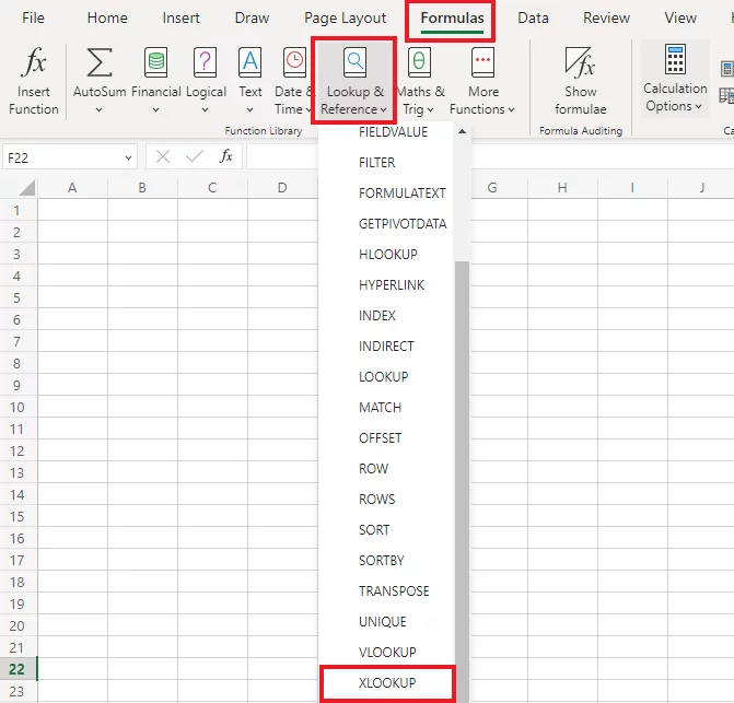
To find the XLOOKUP function from the Functions Library, go as follows.

 

 

Version of Excel

The XLOOKUP function is an advanced function of Excel that is only available to the users of Office 365. Users of the previous Excel versions from 2010 to 2019 will not be able to access the XLOOKUP function.

Brain-Teaser:

But I have the XLOOKUP function employed in my workbook, while I am only subscribed to an older version of Excel.

Such a workbook might be created by an Office 365 user who would have then shared it with you. However, to use the XLOOKUP function in Excel, you must be subscribed to Office 365.

Pro Tip!

Is there some way out you can use the modern-day XLOOKUP function without being an Office 365 user? Yes, through Excel Web.

Log on to your Microsoft OneDrive account and launch Excel online to have access to the latest functions of Excel.

 

Learn more about using One Drive to recover Unsaved Files here.

How is XLOOKUP of use?

It took Microsoft around three decades to come up with a function as wholesome and robust as the XLOOKUP. This function is a successor of the VLOOKUP function and is primarily designed to offer a solution to all the problem areas where VLOOKUP and other functions failed.

Why would you want to use XLOOKUP? Consider the data below.

 

 

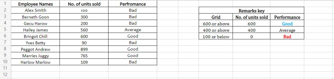
The data consists of employee names alongside the number of items sold by each of them. To the right side of the image, is a key that grades the performance of employees based on the number of units sold by them.

If you want to grade the performance of all the employees as ‘Good’, ‘Average’ or ‘Bad’ – could this be done with a single function?

Yes, the XLOOKUP function. See below.

 

 

Seems like magic? There are many more ways how XLOOKUP can ease your job.

• Use XLOOKUP to fetch a value, array, or range from a given data set.
• Use XLOOKUP to fill grids based on a given criterion in the blink of an eye.

How to do that all? Learn in the article that follows.

XLOOKUP can also help you slim down your data for creating an Excel dashboard. See how to make an Excel dashboard here.

 

XLOOKUP V/s. VLOOKUP

What differentiates XLOOKUP from its predecessor, the VLOOKUP? Below are the four main areas where XLOOKUP outstands the contemporary VLOOKUP function.

 

1.      Vertical and Horizontal Lookup

The VLOOKUP function is designed to perform a vertical lookup only. Take a quick look at the example below to find the difference between a horizontal and a vertical lookup.

 

 

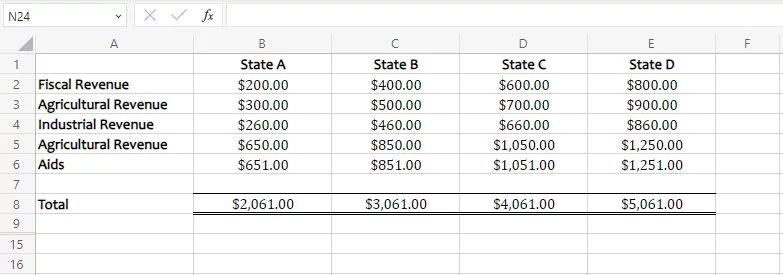
With VLOOKUP, you can find the any sector’s revenue for a particular state (say State B’s fiscal sector revenue) by performing VLOOKUP.

 

 

However, you cannot find any state’s revenue for a particular sector. This is because it requires a horizontal lookup of values which the VLOOKUP function fails to offer.

Using the XLOOKUP function, you can look up the data both ways.

 

                                                                                       

 

Also, excel offers easy ways for column comparison – learn them here.

 

2.      Search Mode & Match Mode

The XLOOKUP function offers two optional arguments that help users to define the match mode. For instance, do you want Excel to return an exact match from the lookup array or an approximate match (higher or smaller values)?

Similarly, search mode allows users to tell if the lookup value needs to be searched for, from the left of the lookup array or the right.

VLOOKUP fails to offer both the above-said features, making it rigid to use.

 

3.      If Not Found Argument

The very common #N/A error of VLOOKUP comes to the screen when Excel fails to find an exact match of what you’re looking for.

While XLOOKUP does no different, it allows users to replace the nasty looking #N/A with any value/dialogue of their choice. You might even choose to leave it vacant.

 

4.      Lookup Array and Return Array can be separately identified

Take a quick look at the data below:

 

The above data is not in a row but in two stacked tables. XLOOKUP can search for a value from such scattered data if the dimensions are compatible. See below.

 

 

However, VLOOKUP cannot handle such datasets. For VLOOKUP to work on such data, the data must be arranged together in a row as below.

 

Pro Tip!

In the above example, if the column for lookup values (Employee ID) is situated after the column for return values (Employee last names), VLOOKUP would again fail to function. The XLOOKUP function allows users to have their lookup array and return array situated anywhere around.

 

XLOOKUP Example 1 – Basic Exact Match

It’s time we delve into examples that demonstrate the uses of the XLOOKUP function. The first example in this article covers the basic function of the XLOOKUP function – seeking an exact match.

 

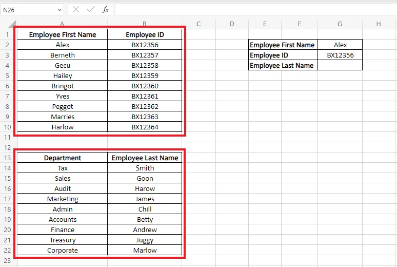
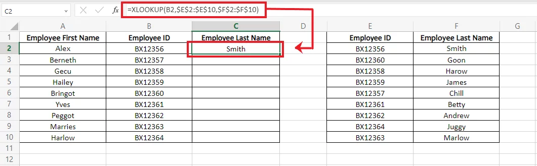
The image below contains data for the employees of an organization.

 

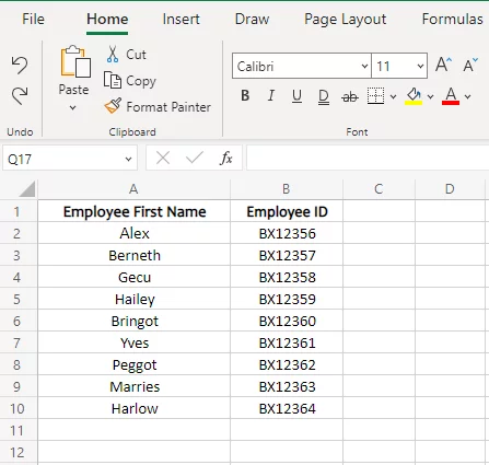
For each employee, the available details include the first name and the employee ID; however, the last name is missing.

Another dataset, as shown below, includes the employee IDs and the respective last names of employees. Now what, copy-pasting?

Do note that the sequence of employee IDs in the second table do not match the sequence in the first table. Copy-pasting the correct last name against each first name might take you ages.

 

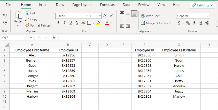
Using the XLOOKUP function under the exact match mode, bringing these two lists together is only about a minute.

Begin writing the XLOOKUP function as follows.

 

 

• The first argument is set to B2, which contains the lookup value – the employee ID against which the last name is required.
• The second argument includes a reference to the lookup_array where the lookup_value is to be looked for. Column H contains the employee ID against the last names and is selected as the lookup_array.
• The third argument consists of the return_array, from where the value is to be returned. We want the last name of employees which are situated in Column I.
• The fourth argument of ‘if not found’ is omitted.
• The fifth argument is omitted as we want an exact match of the employee ID. Excel would have set it to ‘0’ by default.
• The sixth argument is omitted as we want Excel to perform the search from first to last. Upon being omitted, Excel by default sets it to ‘0’.

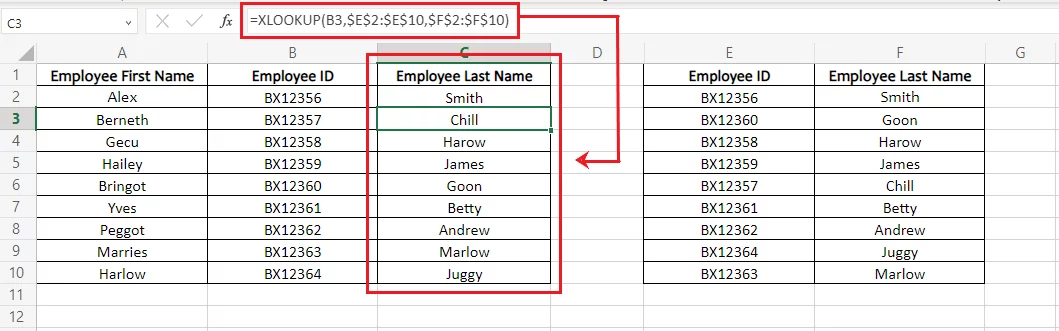
And you’re good to go. Press ‘Enter’ to see the following results.

 

Drag and drop to yield the same results for the remaining employees.

 

XLOOKUP Example 2 – Multiple Values

One main factor that distinguishes XLOOKUP from VLOOKUP is its ability to return not only a single value, but a range of values.

This feature of the XLOOKUP function was much demanded and is of great use. Earlier, to have multiple values returned from a lookup range, multiple VLOOKUP functions were to be combined.

But the very advanced XLOOKUP function can do this in a single formula. See below how.

Let’s expand the example stipulated above to include further detail about employees, as shown below.

 

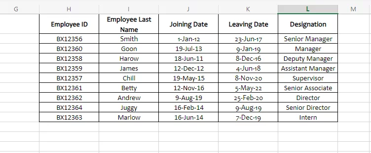
The above data now also constitutes the date of joining and leaving of each employee alongside their designation.

Can we fetch the last name, joining and leaving date, and designation of each employee to the first table all at once? With the XLOOKUP function, yes.

Compose the XLOOKUP function as follows:

 

 

While everything remains the same as the above formula, what has changed?

We have only changed the third argument, return_array from I2:I10 to I2:L10. The range I2:L10 includes four columns. For each employee code (the lookup value) Excel would then return the value of all the corresponding columns from Column I to Column L.

Time to see this in action? See Below.

 

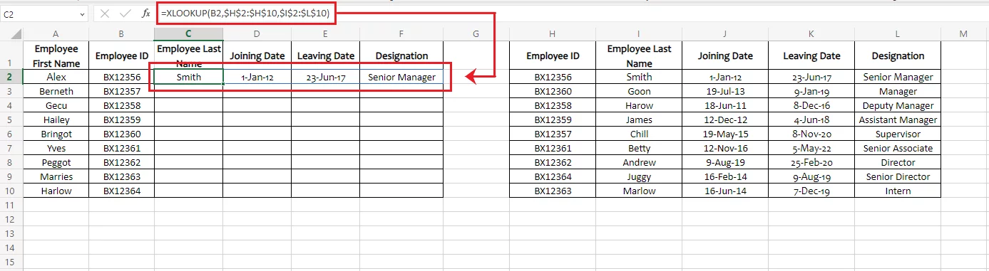
For each employee code, the XLOOKUP function returns multiple cell values from all the specified corresponding columns.

Don’t stop only there. Drag and drop the above function to the entire list to have your data sorted in only a second.

 

 

Point to Ponder: How is this different from the VLOOKUP function?

 

Can VLOOKUP not perform the above operation? The precise answer to this is, that a single VLOOKUP cannot. To fetch more than one value like the above example, you need to operate multiple VLOOKUP functions.

For instance, to fetch all the details for Employee Code BX12360, write the VLOOKUP function as follows:

 

 

Pay close attention to the last argument that specifies the ‘Column’ number of the table from where we want the return value. Here it is set up as ‘2’.

Excel would therefore return the value from the second column (Column I) of the specified table array of H2:L10, which contains Employee last names only.

 

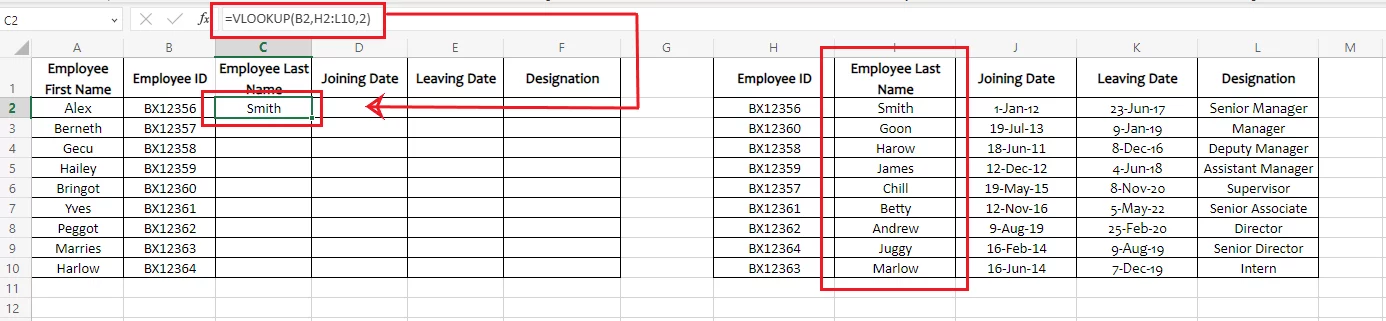
What about the other values? The VLOOKUP functions need to be set up for each of them again and again with the last argument changing to the return value column number.

 

With the XLOOKUP, you can target as many return value columns as desired – that’s when you know how badly XLOOKUP was needed.

 

XLOOKUP Example 3 – Basic Approximate Match

This section is all about the fifth argument of the XLOOKUP function, the match_mode.

You must not have seen this argument to the VLOOKUP function, as this is one of the distinguishing features of the XLOOKUP function.

The XLOOKUP function offers four match modes:

1. Exact Match (0)
2. Exact or larger match (+1)
3. Exact or smaller match (-1)
4. Wild card character (2)

Exact Match returns the exact lookup value from the specified data range. However, if the lookup table doesn’t contain the exact lookup value, Excel would return the #N/A error. This is the same as the VLOOKUP function – the difference is caused by the approximate match modes of XLOOKUP.

Follow the examples below to see how they work.

 

Exact or larger match:

The image below represents the results of a few students from elementary school.

 

Time to allocate Remarks to them all, here is the ‘Remark-key’.

 

Remarks go in line with the marks obtained by each of the above students. But how do allocate them? Let’s not resort to doing so manually.

Set up the XLOOKUP function as follows:

 

 

Let’s quickly breakdown the formula above:

• • B2 contains the score of each student based upon which a remark is sought from the remark key – the lookup value.
  • $G$4:$G$8 contains the score key based on which remarks are to be given – the lookup array.
  • $H$4:$H$8 contains the remarks that are to be returned – the return array.
  • The fourth argument is omitted.
  • The fifth argument, the match mode, is specified as ‘-1’ : Exact Match or Smaller.

 

Why have we set the match mode to exact or smaller?

 

The remarks key says that any student who has obtained 90 or more marks gets ‘Distinction’. Setting the match mode to ‘Exact or Smaller’ tells Excel to look for the exact lookup value of 92 or any smaller value. The next smaller value to 92 in the remarks key is 90. Excel would therefore remark Charlot with ‘Distinction’.

Time to see this in action.

 

Drag and drop the above formula to have the same for the whole list.

 

Pro Tip!

Why have we made the lookup array $G$4:$G$8 and the return array $H$4:$H$8 an absolute reference? As you drag and drop the formula set up in the first cell to the remaining list, Excel would automatically update the cell references, whereas the Remarks key stands static.

To keep the reference to the Remarks key static, add a dollar sign to it to make it static. This way Excel doesn’t change the absolute references when the formula is dragged and dropped.

 

Wildcard character match:

 

How does the match mode work with wildcard characters?

Wildcard characters are used to perform a partial match. The two common wildcard characters are an asterisk (*) and a question mark (*).

Learn more details about wildcard characters in our article on Advanced filters in Excel.

This time let’s sneak peek into a grocery shop that has its items coded to identify their type.

 

Each item has a unique code to it and the quantity of each type of grocery item is written next to it. For example, Kiwi appears on the grocery list but has a unique code to it.

As a store manager, if you instantly want to fetch the quantity of in-stock Kiwi but do not remember the code to it, can this be done using XLOOKUP?

 

Yes, by using the wild card character approximate match.

To quickly sort out the quantity of Kiwi without using the last code to it, let’s set up the XLOOKUP function with a wildcard character as follows:

 

 

The lookup value is set as [Kiwi *]. The wild character, asterisk tells Excel to look out for all values that contain the word Kiwi with any sequence of characters prefixing or suffixing it.

This way, Excel will find out Kiwi even if the ending code to it is not specified.

After a wild character is used, it is important to specify the fifth argument [Match_mode] as 2, which denotes the wild character match.

Press ‘Enter’ to have the results as follows:

 

You may also use the wildcard character of a question mark (?) if the exact sequence and position of the anonymous characters are known.

 

XLOOKUP Example 4 – Complex Criteria

 

We have seen multiple examples where a criterion is specified based upon which XLOOKUP would fetch a value or values for you with a single click.

But what if you have multiple criteria against which the data is to be checked before the targeted figure is returned?

The XLOOKUP function can also be used with multiple criteria. Follows the example to learn how.

 

The image above shows a breakup of state-wise revenue for the four preceding years. The revenue pertains to different sectors, some of which are audited and some unaudited.

If you need to look up data from multiple aspects, how can the XLOOKUP function be set up?

For instance, we need to find the year-wise audited, fiscal revenue of State B. This makes three conditions:

1. Fiscal Revenue
2. State B
3. Audited

 

To specify all these three conditions together in the XLOOKUP formula, begin writing the XLOOKUP function as follows:

 

 

 

Made little sense? We have specified multiple criteria in the lookup array and each criterion would return an array of True (1) or False (0).

As we want these conditions to apply simultaneously, we have used the multiplication sign. Wherever any condition would fail, the result would be 0 – this will be multiplied by the results of other criteria, and the ultimate result would become 0.

Excel would therefore return #N/A if either of the conditions are not met. And if all the criteria turn true, the ultimate result would be 1 for that row, which is the same as our lookup value.

To see this in the formula, let’s break each argument of the above function:

• The first argument is 1, which is the lookup value. We want Excel to lookup for the value 1 i.e. all conditions have been met.
• In the second argument:
  • A2:A5=A11 tells that from the range A2:A5, which represents the revenue sectors, we want A11 (Fiscal Revenue).
  • B2:B5=B11 tells that from the range B2:B5, which represents the state names, we want B11 (State B).
  • C2:C5=C11 tells that from the range C2:C5, which represents the audited/unaudited detail, we want C11 (Audited).

• In the third argument, the return array, we have specified the cell range D2:G5. This contains the revenue for all the years as we want the audited fiscal revenue for all years from 2019 to 2022.

Time to see this in action:

 

What has XLOOKUP done? It has fetched out the year-wise revenue that meets all the three specified criteria i.e. fiscal, audited, and of State B.

That is how you can specify more than one criterion in XLOOKUP at the same time.

 

Pro Tip!

Did you come across the following error?

 

This is because the data to be fetched by XLOOKUP is four columns wide, but the four cells next to the active cell are already occupied. Delete the values from the next three cells and redo the function.

 

Learn more about the spill error through multi-cell and single-cell array formulas.

 

XLOOKUP Example 5 – Two Way Lookup

Conducting search operations in Excel might not always be as easy as looking for a value that meets one specified criterion.

 

Sometimes, you might have two perform a two-way check. For example, look at the data below:

 

The above data of revenue has two dimensions i.e. state and the sector.

Searching out the revenue for any one dimension i.e. the state or the sector, using the XLOOKUP function is a child’s play.

This section discusses how can we seek the revenue for a particular sector and state using the XLOOKUP function in one go.

 

To do so, we need to nest one XLOOKUP function into another. The first XLOOKUP function shall be written as follows:

 

 

B12 consists of the State Name for which we want the data. The above function fetches the revenue for State C.

This function now needs to be nested into another XLOOKUP function that seeks the agricultural revenue sector from the revenues of State C.

 

 

B11 contains the sector name (Agricultural Revenue) for which we need State C’s revenue. The lookup array is substituted by the previous XLOOKUP function that fetched the revenue for State C only.

 

This way Excel performs a two-way search. The nested XLOOKUP function sorts out the revenue for State C only. The outer XLOOKUP function then sorts out the agricultural sector revenue from State B revenues.

 

XLOOKUP Example 6 – Not Found Message

 

If you have ever used any of the lookup functions, you must be familiar with the very irritating #N/A error posed by Excel time and time again.

Excel poses the #N/A error message when it fails to find the lookup value in the lookup array, and hence there is no value to return.

The VLOOKUP function doesn’t offer an in-built solution to cater to this problem. The max you can do is to nest your function into an IF function to display a message of your choice instead of the #N/A.

Like all the other inherent problems of the VLOOKUP function, the XLOOKUP function brings an in-built solution to this problem as well. How? Through the fourth argument of the XLOOKUP function.

If Excel fails to find the lookup value in the lookup array, it gives back the value specified by you as the fourth argument rather than an #N/A message.

Let’s see the above in action through the example below.

The data below is about a few regions and their states.

 

Let’s take a quick turn to populate the third column to it, which is for the country codes using the key below.

 

Using the XLOOKUP function, the country code for each region can be sought as follows:

 

The above function tells Excel to look out for the states in the country code key and return the respective country code for each region. The country code key doesn’t have all the states, as shown in the data.

Note: The lookup array and return array have an absolute reference, and the fourth argument is omitted.

Excel is going to have a hard time finding all the lookup values in the lookup array.

Hit Enter and drag and drop to have the results as follows:

 

For some regions, Excel returns the country codes based on the state. However, for the other, Excel only returns an #N/A error.

 

How to get rid of this?

 

If you do not want a stubborn #N/A error to appear in such circumstances, you can input a dialogue of your choice. To do so, change the above XLOOKUP function as follows:

 

Adding the fourth (if_not_found) argument tells Excel to display the text in quotation marks instead of the #N/A error whenever a lookup value is not found.

Hit enter and run the drag and drop functionality once again to yield results as follows:

 

Lessen the anxiety in your eyes by getting rid of the alerting #N/A error of the lookup functions and replace it with any dialogue of your liking. You might even set it to nothing by designing the fourth argument as “”.

 

Must note!

If you want to set a text value in place of the if_not_found argument, do not forget to enclose it in quotation marks as shown above. Excel would otherwise fail to identify the text value. You can also refer to another cell as the if_not_found argument.

Pro Tip:

The fourth argument of the XLOOKUP function is optional and can be omitted. When omitted, Excel returns the #N/A error.

 

XLOOKUP Troubleshooting

 

There are a variety of errors the XLOOKUP function might pose while you continue to twitch it in different ways. Once you know what each error has to say, resolving it shouldn’t take you a great deal of effort.

#REF Error

The very annoying reference error is set forth by the XLOOKUP function when it is being operated in two or more workbooks at the same time. This might be the case when the lookup array and the return array reside in one workbook, and the XLOOKUP is employed in another workbook.

That’s no big deal as Excel can handle that effortlessly. However, for this to be done, both the workbooks must be simultaneously launched in the background. If either of the workbooks is shut, Excel would end up returning the #REF error.

Simply open both the workbooks to get rid of the said error.

 

#VALUE Error

The #VALUE error posed by Excel is an indication that the lookup array and the return array specified by you are not compatible in terms of dimensions.

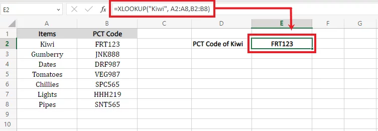
For example, if your lookup array has 7 rows but your return array is only 5 rows long, Excel would give back a #VALUE Error. See below:

 

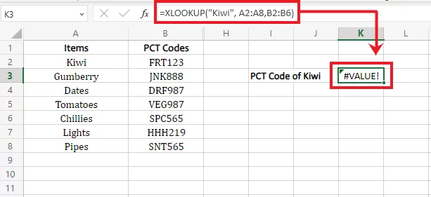
Excel fails to return the PCT Code for Kiwi because of incompatible dimensions of both arrays. Change the return array to make it parallel to the lookup array to see the #VALUE error vanish away.

The return array is changed from B2:B6 to B2:B8 – compatible with the lookup array of A2:A8.

 

Absolute References

This is not a problem with Excel but a problem with the drag-and-drop function. See the example below.

Here we have set the formula for Cell C2 by setting the Marks key as the lookup array and the remarks key as the return array.

 

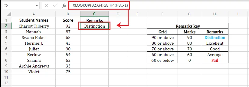
The formula runs perfectly well for the first cell. However, drag and drop it down to the entire list, and the results would distort as follows.

 

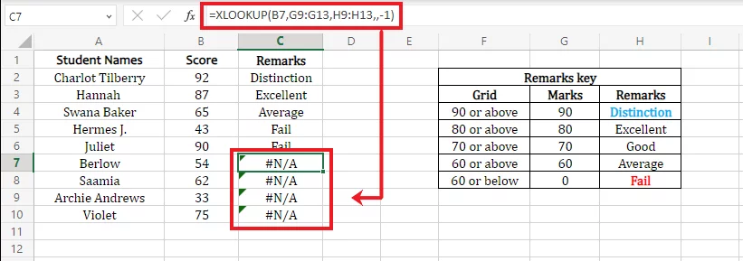
The #N/A error tells the lookup value is not found. This is because when dragged and dropped, Excel automatically updates the cell references, and the lookup array and the return array have changed.

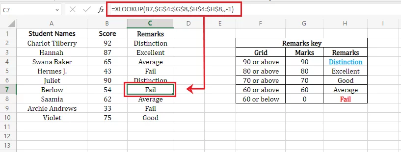
Turn the lookup array and the return array into absolute references by navigating the cursor to each cell reference in the formula bar and pressing the F4 Key. See how the results change.

 

Conclusion

In the fast-paced world of today, smart and swift functions like the XLOOKUP are a necessity. Going through the above article and understanding the functionality of each example therein can help you master the XLOOKUP function with sheer ease.