Compare Two Columns In Excel (Ultimate Guide!)

When dealing with Data analytics, comparing data populated in two or more columns is common practice.

Manually comparing data could take hours or even days, depending on the amount of the data in question.

But when it comes to using Excel, you can expect data work to be done in a matter of minutes

The same is true for comparing two columns in Excel.

When we cover this on our Excel intro course, we spend a lot of time on the topic as understanding this is key to Excel!

Why Compare Columns in Excel?

You may want to Compare Columns in Excel to find matching, or non matching data, or specific information.

The first step to compare columns typically involves comparing data by sorting it into two or more adjacent columns.

This is one of the quickest techniques in Excel and can compare any amount of data in less than a second.

Exact Row Match

When comparing two cells, Excel matches the same row of the first column against the second column to find the similarities or differences.

The top four methods for comparing two columns are listed below:

• Method # 1: Compare two columns using a Simple Formula
• Method # 2: Compare two columns using IF Function
• Method # 3: Compare two columns using EXACT Function
• Method # 4: Compare two columns using conditional formatting

Let’s explore these methods and related examples below:

Compare Two Columns Using a Simple Formula

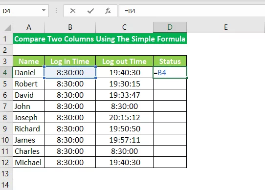
Look at the following datasheet. It reflects the record of 10 employees in an organization displaying their log-in and log-out time.

Column A represents the names of the employees, whereas Column B and Column C display their log-in and log-out times, respectively.

In this example, our objective will be to highlight the employees who forgot to log out using a simple Microsoft Excel technique.

Since the office timings begin from 8:30, so the employees who didn’t log out will have the same log-in and log-out time.

Let’s now compare the columns and see the results.

We use the comparison operator “=” (equal to) to find the exact match in two columns. It is used as follows:

Step 1

In cell D4, enter the operator “=” in the formula bar and select cell B4.

Step 2

Enter the “=” operator again, followed by selecting cell C4.

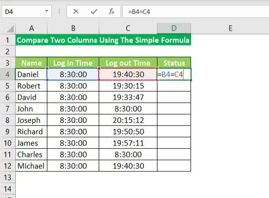
Step 3

Now press the “Enter” key. You get a “false” value in return; this implies that the value in cell B4 is not equal to that of cell C4.

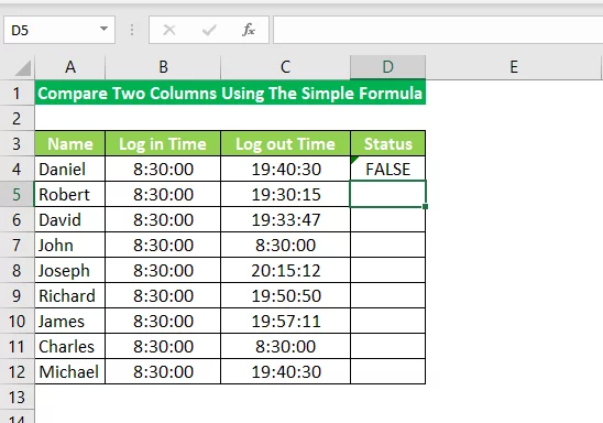
Step 4

Now drag the cell handle or copy-paste the formula to the remaining cells.

The output will be either “True” or “False,” as shown in the figure above.

Assuming that the column B and column C have the same values, you obtain “True” in the result and vice versa.

Here, ‘True’ means that the log-in and log-out time match, which in turn suggests that the employee forgot to log out.

In contrast, False means that the log-in and log-out entries do not match each other.

Hence, as evident from the gif, two employees, John and Charles, did not log out properly.

Note: You may employ the filter function to immediately sort out the rows with the corresponding value ‘True’ in column D.

This will help you filter out the employees who forgot to log out.

Compare Two Columns Using the IF Function

Considering the above example again, let’s now compare the two columns, B and C, using the IF Function.

The result of the comparison must be something like this:

• • “Forgot log out” if the employee forgot to log out
  • “OK,” if the employee logs out properly

The syntax of the IF function for this comparison is as follows:

=IF (B4=C4,“Forgot log out”,“Ok”)

Since the IF function makes a logical comparison between two values, let’s see how the formula works before getting into its example.

The IF Function compares two columns, and if they are matching values, the Function returns “True”; otherwise, it returns “False.” Now for every “True” value, it displays a specific text.

In this case, Microsoft Excel displays the message, “Forgot log out,” for every true argument.

Similarly, the formula is set to return the message “Ok” for every “False” value.

If the technical language here is a bit confusing, we cover logical functions from the ground up in our courses.

Let’s apply it to our data as follows:

Step 1

Put the above IF Function in cell E4 and press Enter to get the output.

Step 2

Drag the cell handle or copy-paste the cell formula into the remaining cells to obtain the output.

The Function displays Forgot log-out message where both the cells have matching values, and displays OK, where the same values are different.

This Function can be pretty helpful when dealing with a large list of items and matching their properties.

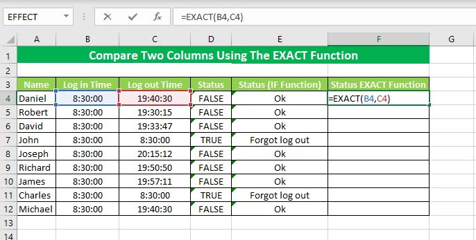
Compare Two Columns Using the EXACT Function

Considering the data in the above example again, let’s use the EXACT Function to compare two columns.

The syntax of the EXACT Function is as follows:

=EXACT (B4, C4)

Step 1

Put the above Exact formula in the output cell F4.

Step 2

Press the Enter key to get the following result.

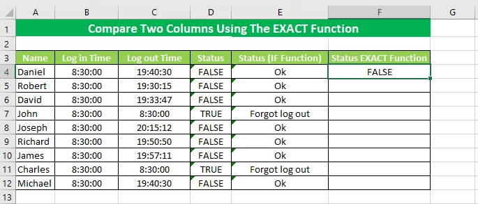
Step 3

Drag the cell handle to copy the formula in the remaining cells.

Comparing both columns with the EXACT Function shows two true cases where John and Charles forgot to log out properly.

Tip: Note that the Exact Function is case sensitive, i.e., treats uppercase and lowercase characters differently.

Comparing Two Columns Under Effect of EXACT Function’s Case Sensitivity

To see how the EXACT Function works with case sensitive data, let’s see the example below:

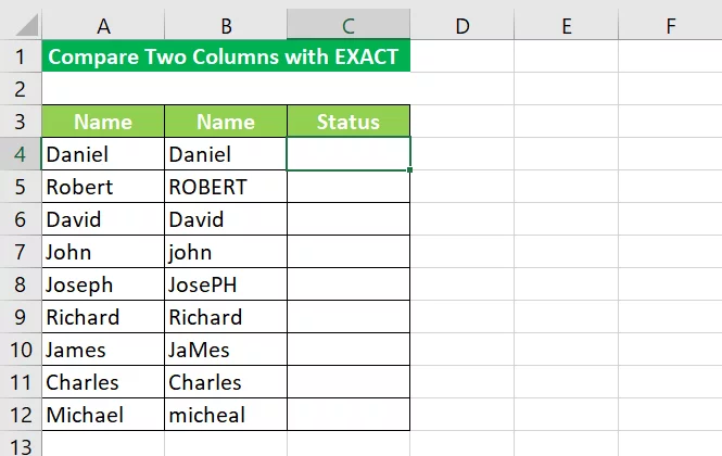
Using the same data as in the above examples, we changed the letter case of the names.

Let’s now compare both the columns using the EXACT Function. The syntax of the EXACT Function looks something like this:

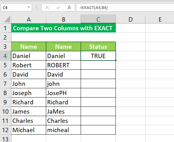
=EXACT (A4, B4)

Step 1

Insert the syntax in the formula bar by selecting cell E4 and pressing Enter. The result will be displayed in the cell as:

Step 2

Drag the cell handle to copy the EXACT formula in the remaining cells.

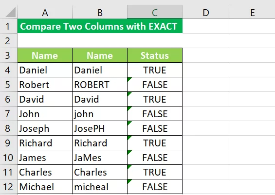
As evident from the image above, the EXACT Function returns “False” when the casing of Cell A is different from Cell B and vice versa.

Compare Two Columns Using Conditional Formatting

Another feasible method is using conditional formatting. It comes in handy when you want to compare data in two columns and do not want the result to be displayed in the third column. You can find the matching entries within the two columns using conditional formatting.

Consider the following example:

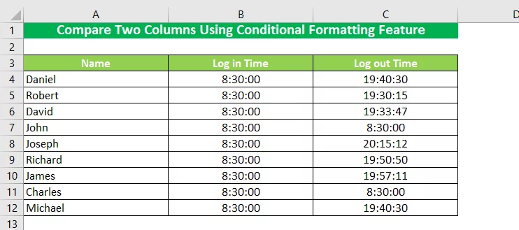
To highlight the matching columns in the above image, follow the steps given below:

Step 1

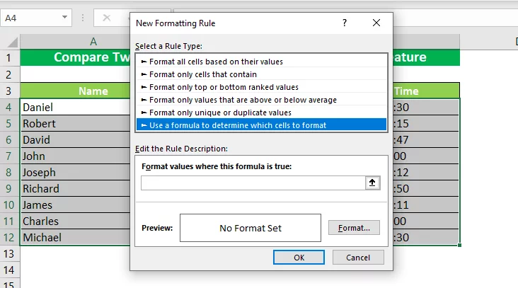
CTRL+A to select the entire data. In the “Home” tab, select “Conditional formatting.” From the drop-down list, select “New Rule,” and the “New Formatting Rule” window appears.

Step 2   

From the new formatting rule dialog box, select “Use a formula to determine which cells to format.” The drop-down list will expand to get the formula for the cell formatting.

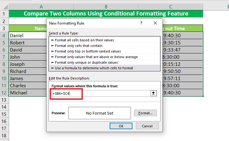
Step 3

Now enter the formula “=$B4=$C4” under the “edit the rule description.”

Step 4

Once done, click the “format” button, and a Format Cell window will appear. From the format Cell window, select the “Fill” option from the top menu and select the color that you want to fill in the identical columns. Click the “Ok” button twice, and you’re done.

The matching entries of column B and C are highlighted as shown in the figure below:

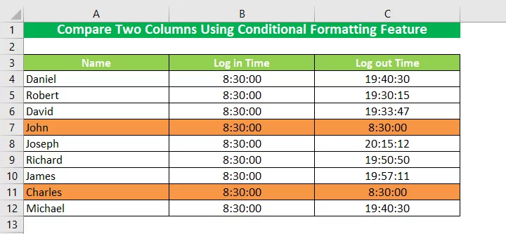
It is clear from the results that the log-in and log-out columns of John and Charles are identical, indicating that their log-out time was different than others.

This is how you can use the conditional formatting feature to compare data using your customized formulas to get the desired results.

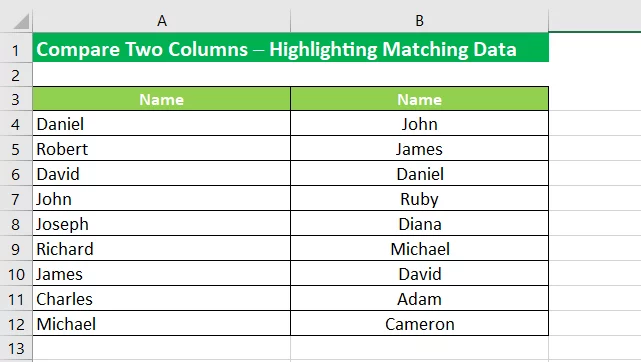
Highlight Matching Data

Like the method above, you can use conditional formatting to compare two columns by comparing each cell of both columns and not involving a row-by-row comparison.

Consider the following example:

To highlight the matching data in two columns, follow these steps:

Step 1

Select the entire data set and from the “Home” tab, select “Conditional formatting.” In the drop-down list, hover the cursor over the “Highlight Cell Rules” and select “Duplicate Values” from the list. From the Duplicate Values dialog box, select the color scheme that fills the cell matching in both columns. Once done, press OK.

The result will be something like in the image below:

 

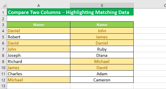
The conditional formatting function highlights the matching entries in both columns.

Tip: Must note how the Conditional Formatting duplicate rule is not case sensitive. Therefore, conditional formatting can be used to compare two columns if case sensitivity is not your concern.

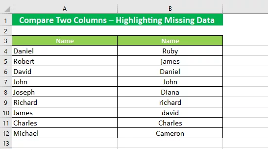
Find Missing Data

You can use any of the two methods below to find any mismatched data in your column set. These involve Excel formulas and formatting features making the process quick and fun.

1 – Finding Mismatched Data Using Formula

The first method is based on the use of a formula to find mismatched values. For that, let’s see the example below.

Step 1

Select the entire data set. Go to the “Home” tab and click the “Conditional formatting” tab. From the drop-down list, select the “New Rule” option and from the “New Formatting Rule” window, select “use a formula to determine which cells to format.”

Step 2

To highlight the mismatched values, enter the following formula in the Edit formatting rule dialogue box under the box that reads “Format values where this formula is true”.

=$A4<>$B4

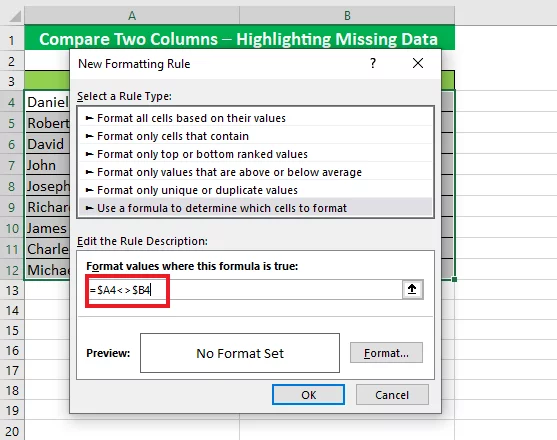
Step 3

Click the “Format” button to select your desired color for mismatched data, and choose the color from the “Format Cell” window. Press the “Ok” button twice, and tada! You’re done.

The highlighted cells are visible in the image below:

In the above image, all the mismatching rows in both columns have been highlighted using Conditional Formatting, whereas the matching data remains unchanged.

2 – Finding Mismatched Data Using Conditional Formatting

Excel also offers features that help you find data in a single column. We use conditional formatting for this method as well.

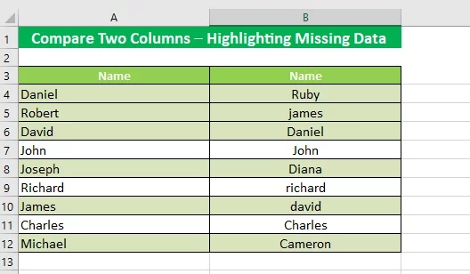
Consider the following example:

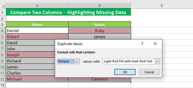
Step 1

Select the entire data. Go to the “Home” tab and then select the “Conditional Formatting” tab. Move the cursor on the “Highlight Cell Rules” and select the “Duplicate Values” option from the drop-down list. You will see the Duplicate Values dialog box on your screen as follows:

Step 2

Select the option “Unique” and specify the formatting for those unique data.

Step 3

Press “Ok” to get the results.

The image displays unique data highlighted in both columns as below:

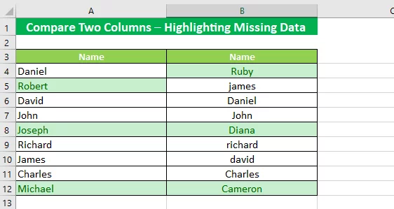
Since the Conditional Formatting feature is not case sensitive, it considers “David” and “david” the same entries. However, if your work calls for dealing with case-sensitive data, you can go for the other diverse options mentioned in this article.

VLOOKUP

When you want to compare two columns in Excel, the VLOOKUP function is the king. It offers multiple options to compare data.

Let us see how to use the VLOOKUP function to its full potential while comparing two columns in Excel.

Consider the following example:

 

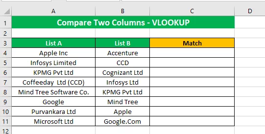
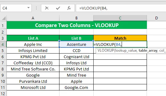
The above image displays two lists of various companies’ names. We will use the VLOOKUP Function to compare multiple columns and find the matching entries.

Step 1

Let us suppose we want to compare List A to List B to find the common names in both columns. Here is how we can use the VLOOKUP function for the said purpose.

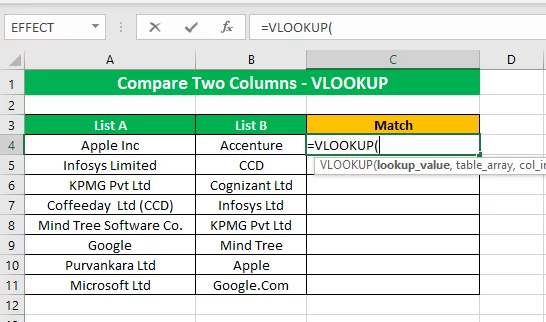
Step 2

Insert cell B4 in the VLOOKUP formula as we want the values in List B to be looked up.

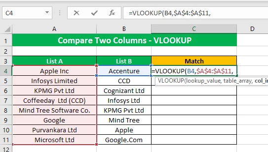
Step 3

In the next argument, the Table array (where the values are to be looked up for) is set to List A. Select the range of cells from A4 to A11 and make it an absolute cell reference by pressing F4.

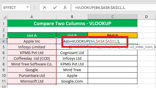
Step 4

The next argument is the “Col Index Num,” number of the column from left to right from which the result is to be obtained. Since List A consists of only one column, so the “Col Index Num” will be 1. Insert this value in the Function.

Step 5

The fourth and last argument to the VLOOKUP function is an optional one. You may set it to FALSE or leave it omitted to Excel to set it to FALSE by default.

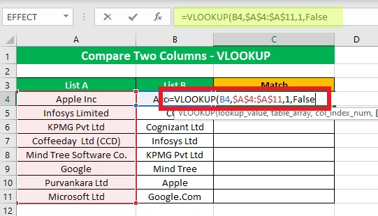
Step 6

Once you’re done with the Function, close the bracket and press “Enter” to get the results.

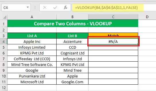
It is clear from the result that the cell value Accenture is not available in List A. #N/A equates to the fact that the values do not match.

Step 7

Drag the cell handle and copy the VLOOKUP function in the remaining cells.

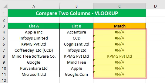
VLOOKUP facilitates a quick comparison of data populated within multiple columns.

However, in the case of ‘no match, it returns the error “#N/A”. This may confuse inexperienced users, making them think that something is wrong with the formula.

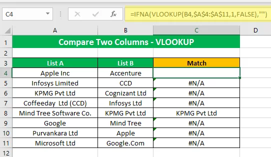
To remove this Error message, replace it with a blank by using the IFNA function. The syntax of the IFNA function for this comparison will be something like this:

=IFNA(=VLOOKUP(B4,$A$4:$A$11,1,FALSE),””)

 

Step 8

Insert the IFNA function in the previous example and press “Enter.”

Step 9

Drag the cell handle to copy-paste the IFNA function in the remaining cells. The result should look something like this:

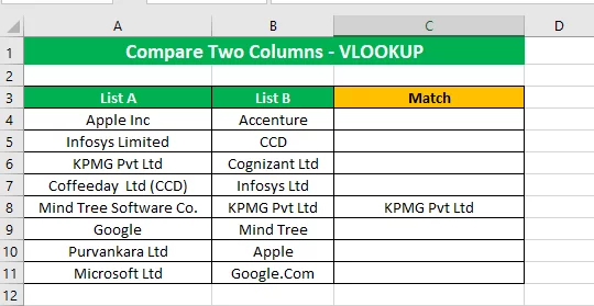
It is evident from the image above that “KPMG Pvt Ltd” is the only company name that exactly matches both column A and column B.

Using VLOOKUP For Partially Comparing Two Columns In Excel

In the above example, a few names exist in both the column A and column B, but are followed by suffixes or prefixes.

Until the values are in absolute conformity (letting aside the letter case), Excel matching or comparing functions would fail to fetch the desired results.

However, the VLOOKUP function has the capability of handling such situations using the “Wildcard Characters.”

You can use the wildcard character (*) that enables the VLOOKUP Function to look up values before and after the selected data. Let us see the use of (*) to get the desired match.

Step 1

Modify the above formula and add (*) as given below:

=IFNA(VLOOKUP(“*”&B4&”*”,$A$4:$A$11,1,FALSE),””)

Step 2

Drag the cell handle to copy-paste the formula into all the cells. The result will look something like this:

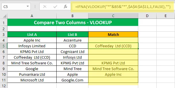
Before using the wildcard character ‘asterisk,’ Excel returned only one match, but upon using the wildcard character, the formula returned three more matches. Weird, no?

Let’s see the science behind this change.

The wildcard character asterisk matches any number of characters. As we applied the asterisk before and after the data value of each cell of list B, it returned every entry from List A that had the text string from List B.

For example, cell B5 contains CCD, whereas A7 contains “Coffeeday Ltd (CCD)”. Using the wildcard character ‘asterisk’ matches and gives back all results from Column A that have the text string CCD.

The same is true for “Mind Tree” and “Apple” present in B9 and B10.

Here’s how seamless the process is.

 

Pull Matching Data

Comparing multiple columns in Excel is a normal practice and is usually utilized in making administrative decisions.

By comparing the data columns, you can pull out information to analyze the data, and the VLOOKUP function is extremely helpful when it comes to matching data.

Let us now see how you can use VLOOKUP to draw the matching data in another column.

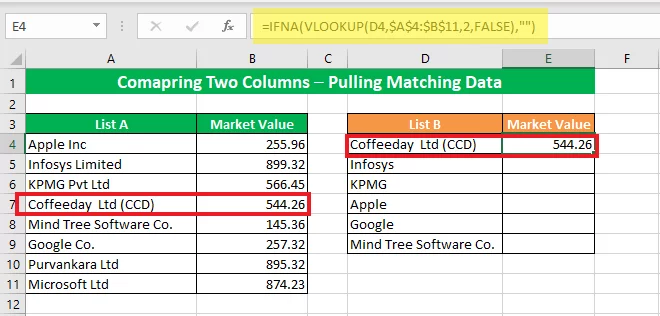
Consider the following example:

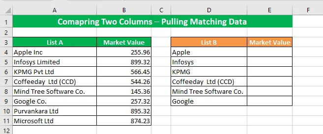
List A consists of companies’ names, whereas the Market Value column contains their market price, respectively.

Suppose we want to fetch the market value for List B.

To do that, we will use the VLOOKUP Function to find values in List A and then fetch the corresponding market value from List B.

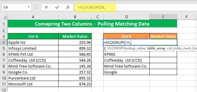
Step 1

Insert the VLOOKUP formula in cell E4.

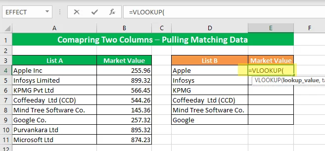
Step 2

We want to look up the market value of the companies from List B, so we select cell D4 as the lookup value.

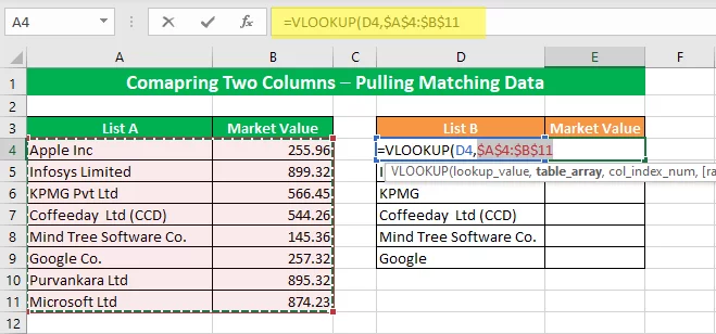
Step 3

Since we want to find the market values of the selective companies from List A, we select the “Table array” range from A4 to B11 and make the cell reference absolute by pressing F4.

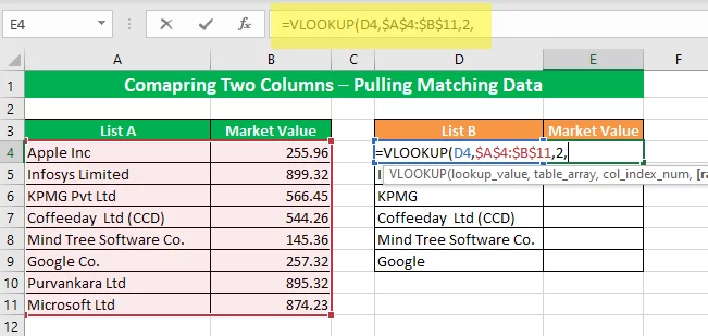
Step 4

To fetch the market price of the selective companies, we insert the column index of the market value data column, which is 2.

Notably, the Column Index is counted from left to right in the selected table array.

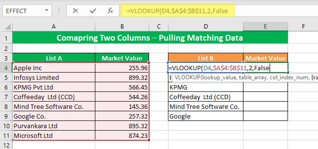
Step 5

We enter False or 0 as the last argument in the VLOOKUP Function for an exact match to obtain the results.

Step 6

Once done with the VLOOKUP formula, close the bracket. Since we have learned in the previous example that the VLOOKUP function returns a #Num error for a mismatch, you may want to nest the above Function into the IFNA function for better results.

The formula will look something like this:

=IFNA(VLOOKUP(D4,$A$4:$B$11,2,False),””)

Now put this formula in cell E4 and press “Enter” to get the results.

Step 7

Drag the cell handle to copy-paste the VLOOKUP formula into all the cells.

 

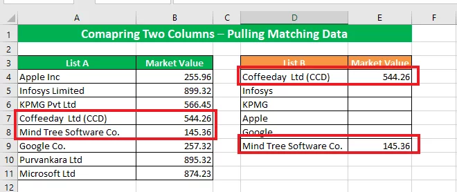
Pulling Matching Data

The above example represents the instance where the VLOOKUP function matched and returned the values that were an absolute match.

However, it did not work the same for “Apple” and “Apple Inc.” Here’s what you can do to look up values having prefixes or suffixes.

In the previous example, we learned how to use the wildcard characters to fetch the partially matched cell values. We can apply the same wildcard character (*) here to fetch the partially matched data while comparing two columns in Excel.

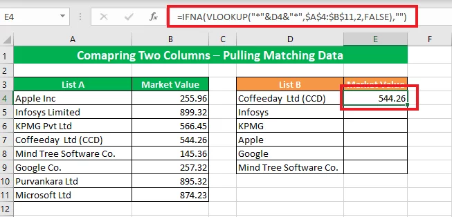
The formula for fetching partially matched data looks like:

=IFNA(VLOOKUP(“*”&D4&”*”,$A$4:$B$11,2,FALSE),””)

Step 1

Put the above formula in cell E4 and press “Enter” to get the result.

Step 2

Drag the cell handle and copy-paste the above formula into the remaining cell to get the partially matched data.

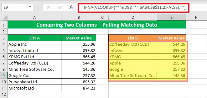
The above image shows how the VLOOKUP function finds data with partial matching using the asterisk (*) character.

Cell D5 contains the value “Infosys,” whereas A5 contains the value” Infosys Limited.”

Using the asterisk (*), VLOOKUP fetches those values even if they are not an absolute match.

Here’s a glance at how you can pull the matching data using the VLOOKUP function while comparing two columns in Excel.

 

Example Of Pulling Data by Comparing Two Columns

Since we are now well versed with the methods of comparison of two columns in Excel and pulling data in the third column using the VLOOKUP function, let us use the techniques altogether.

Consider the following example.

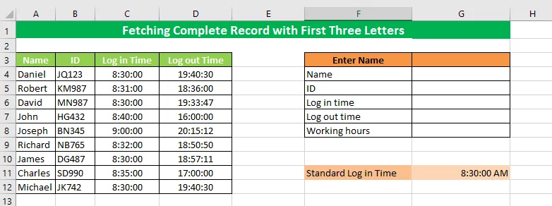
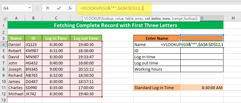
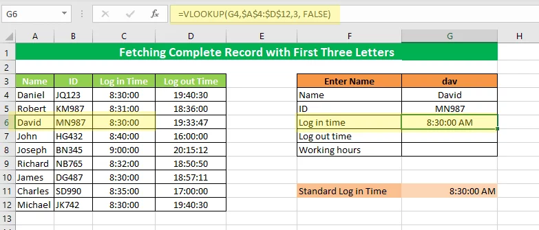
The above example shows employees’ records of their log-in and log-out time along with their company’s ID. Using this template, you can fetch the record of any employee by using the first three letters of their name.

Let us see how it works as below:

Step 1

Since the template works by using the first three letters of the employee’s name, the focus is placed on the Name column, i.e., G4.

To obtain results with only the first three letters of the employee’s name, the VLOOKUP function needs to work together with an asterisk.

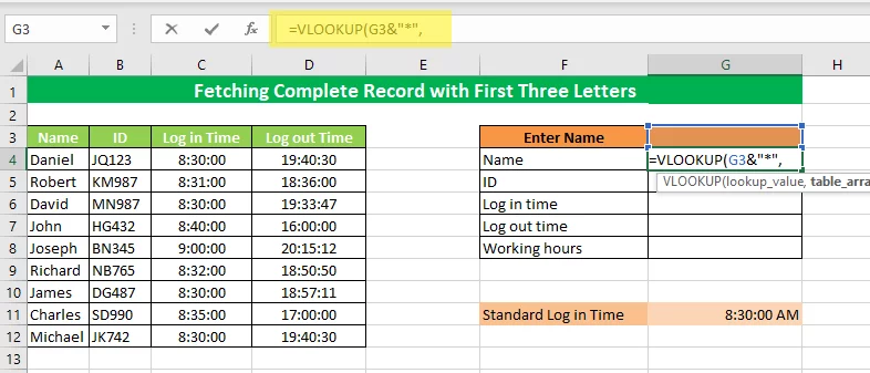
The first argument of the VLOOKUP function will look something like this:

=VLOOKUP (G3&”*”,

This argument is for the value of cell G3 with any number of letters on its right side. Insert the Function in the cell as:

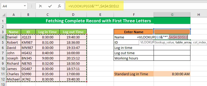
Step 2

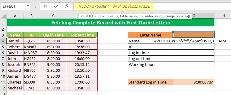
For the table array, select the array range from A4 to D12 and turn it into an absolute reference.

Step 3

Since we want to look up the Name column, which has the index 1 in the selected column array, the “Col_index_Num” is set to 1.

Step 4

For an exact match of the Name value, we put “False” as the last argument in the VLOOKUP function.

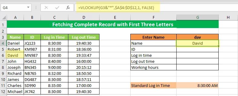
Step 5

Once done with the VLOOKUP function, close the bracket and press Enter. Entering the first three letters in cell G3, Excel gives back the following results.

Step 6

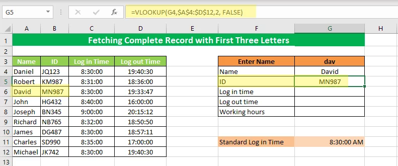
For fetching the ID, let’s consider the value of G4 as the Look_up value. Since we are looking for an ID value that has Col_Ind_Num 2 in the selected table array, the Col_Ind argument is set to 2.

And for an exact match, we will add “FALSE” to the VLOOKUP function. The VLOOKUP function for fetching ID values will look like this:

=VLOOKUP (G4,$A$4:$D$12,2, FALSE)

Put the above formula in cell G5 and press Enter.

Step 7

For Log In time, we will use the same formula as we used for ID value; the only difference will be the Col_Ind number. It will be 3 for log-in time. The Function will look like this:

=VLOOKUP (G4,$A$4:$D$12,3, FALSE)

Put the above formula in cell G6 and press Enter.

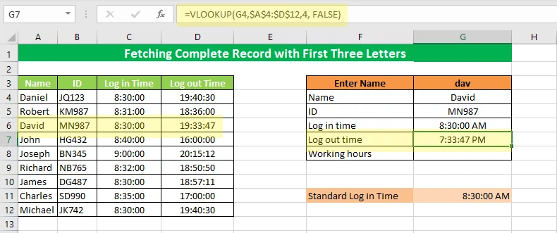
Step 8

For fetching Log out time, use the same formula with Col-Ind_Number as 4. It will look like this:

=VLOOKUP (G4,$A$4:$D$12,4, FALSE)

Put the formula in cell G7 and press Enter.

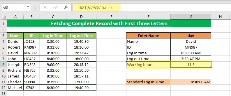
Step 9

The Working hours reflect the total time that an employee spends in the office. To calculate working hours, we will subtract the Log out time from the log-in time.

To do so, let’s bring to use the TEXT function. The syntax for the TEXT function for calculating working hours would take shape as follows.

=TEXT (G7-G6, “h:m”)

 

Put the above formula in cell G8 and press Enter.

Step 10

The Conditional Formatting feature makes an appropriate choice to format the cell by comparing all the cells.

If any employee logs in after the standard log-in time, the template should reflect it as follows.

Here is how the template works. It compares multiple columns and fetches the required data using the VLOOKUP Function.

Not only that, it automatically calculates the working hours for each employee and indicates if any employee logged in late by changing the color of the cell.

Use Cases of Comparing Columns

Comparing two data columns having 5 or 10 entries is a piece of cake.

But what if you have thousands of data entries in both columns?

In case you are a beginner, let’s first familiarize ourselves with what the comparison of two columns in Excel is used for.

We have listed some use cases below:

• Maybe you want to find the top-selling mobile phones at your store – you can compare the sales of mobile phone data to find the top selling phone.
• Perhaps you want to find out which of your favorite football players qualified for a tournament – here you can compare your favorite players with qualified players and find out.
• If you want to know the availability of certain gadgets from a huge list of items at your store – you can fetch the data by comparing your required items with the store inventory.
• Similarly, you can find out the share price of your stock by comparing it with the stock data in a few clicks!

There are hundreds of other cases which involve comparing columns.

Troubleshooting:

Comparing columns in Excel is a dynamic exercise – you can bring to your use a wide variety of functions, formulas, and tools to help the job.

However, if you get improper results while comparing two columns in Excel using the functions demonstrated above, do check for the following common problems.

• • #N/A Error

It is not an error in nature. Instead, it is a system message returned when you use the VLOOKUP Function to compare two columns for an exact match. In case of a mismatch, the VLOOKUP function returns the message #N/A.

To avoid such error messages, you can use the IFNA function to replace this error message with an empty cell instead.

The syntax for the IFNA function is as follows:

=IFNA (VLOOKUP (lookup_value, table_array, column_index_num, [range_lookup]),””)

Let’s recap on how to resolve this issue quickly.

• • #NAME? Error

If you get this error while using the VLOOKUP function, check out the VLOOKUP function syntax. One of the possible reasons for this error is the wrong spellings of “True” or “False” in the VLOOKUP function arguments.

• • #VALUE Error

Finding a #VALUE error indicates that you might have made some mistake while writing the VLOOKUP argument. Removing the syntax error can rid you of this error message.

Conclusion:

Excel provides a variety of methods and functions to compare two columns, including the use of a simple operator “=”, the EXACT Function, the IF Function, and the Conditional Formatting feature

Not limited to the above, you may use the VLOOKUP function for performing column comparisons in Excel.

The VLOOKUP function is undoubtedly one of the most powerful functions of Excel to compare two columns in Excel and fetch matching or partially matching data into another column.

Practice the techniques discussed above to become an Excel whiz in no time. Happy Excel Exploring!

For more on Excel, check out our Using AI With Excel article here!