
How To Use A Checkbox In Excel
Contents
Checkboxes are one of the clearest visual indicators of all time.
You can insert multiple checkboxes, to make your spreadsheets more interactive.
An Excel form control tick box is easier, in some instances, to use than ActiveX controls.
The reason being that you don’t need to use VBA with form controls.
We have been running Excel London training courses for over 20 years and this is one topic people always find useful!
What is a Checkbox?
A Checkbox is a small square, which can be either checked or unchecked.
This often gets confused with check marks, which are simple “✔” characters in Excel.
You will often see multiple checkboxes on web forms or when filling in surveys.
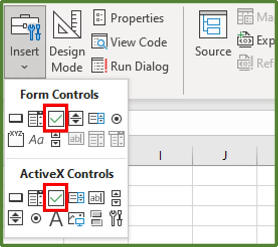
There are two types of checkboxes one can utilise in Excel.
The form control checkbox relies on formulas and linked cells for functionality.
The ActiveX checkbox relies on VBA for functionality. In this tutorial we are going to focus on form control checkboxes.
Checkboxes are also very useful for creating heat maps, a very underrated visualisation tool!
Checkbox Use Cases
You can use checkboxes to create:
- simple to-do lists
- simple daily and weekly planners
- interactive charts, reports and dashboards
Using The Developer Tab
You have to add the Developer Tab to the excel ribbon first, in order to insert and use checkboxes.
Step 1:
To do this, go to the File Tab and select Options.
This will open up the Excel Options Dialog Box. Select the Customize Ribbon option.
Ensure the Developer option is checked.
Click Ok.
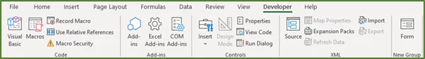
The Developer Tab will now be on the excel ribbon.
The part we are interested in is the control tab!
Adding A Checkbox To Your Sheet
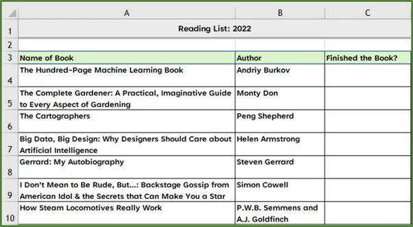
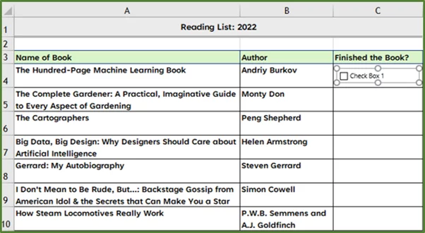
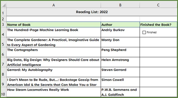
In our first example, a hypothetical student has his desired reading list for 2022 on a spreadsheet.
As soon as he finishes a book on the list, he wants to tick it off, using a checkbox.
The source data is shown below.
Step 1:
So go to the Developer Tab, and in the Control Tab, click Insert.
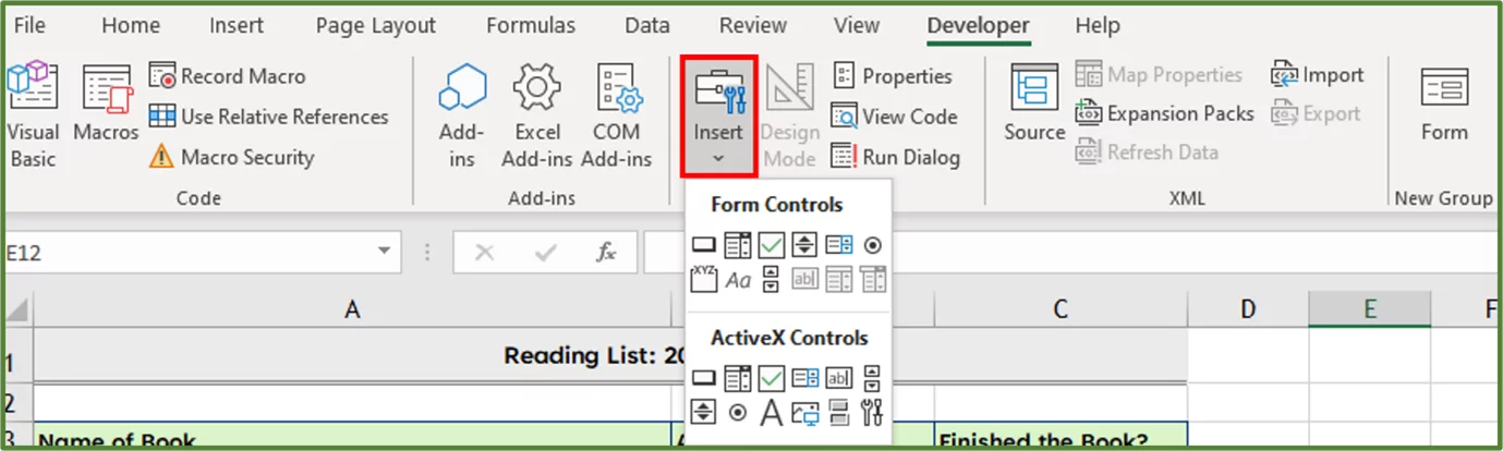
In the Format Control dialog box section, select Check Box.
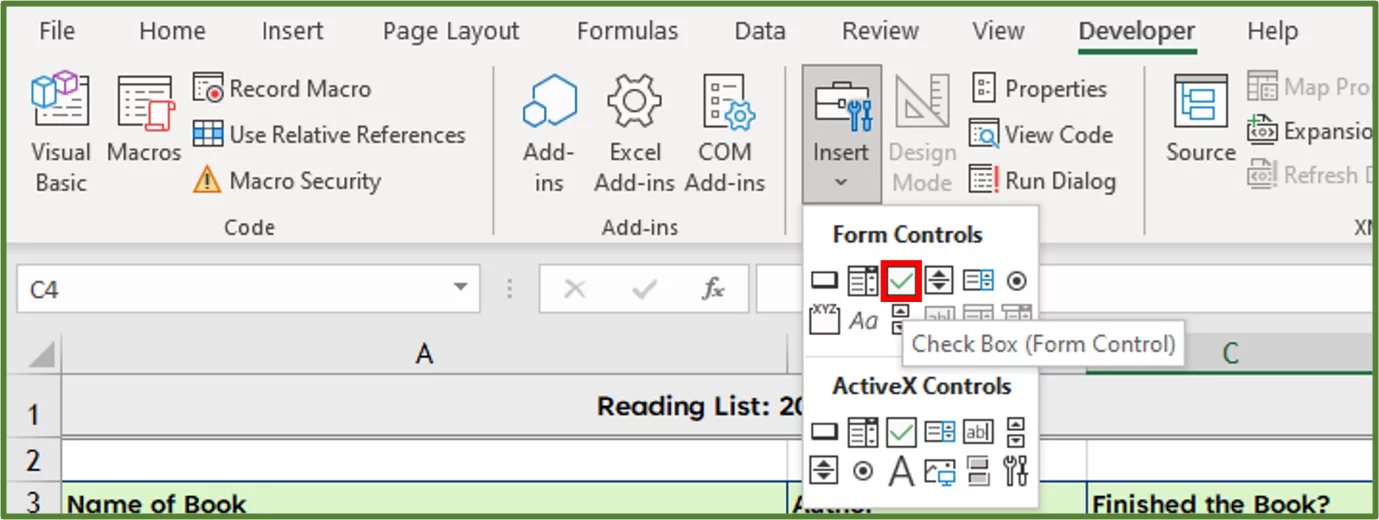
Draw a checkbox on the sheet (you can place it anywhere you like), in this case it is in cell C4.
Step 2:
Right-click the checkbox and select Edit Text.
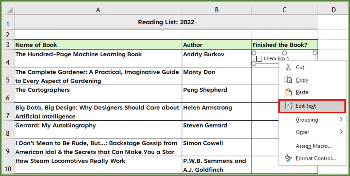
Now you can either delete the text entirely, or in this case we will type Finished.
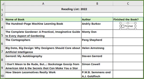
Now working with a checkbox can be a bit tricky at first.
In order to select the checkbox, hold the CTRL key on your keyboard first and then left-click the checkbox.
You can reposition the checkbox by selecting it and then using the arrow keys on your keyboard.
Additionally, you can resize the checkbox by dragging the handles.
We have resized and repositioned the checkbox as shown below.
Step 3:
Now you can copy the checkbox to the other cells, by selecting cell C4 and then dragging down the column.
Click on another cell to deselect everything.
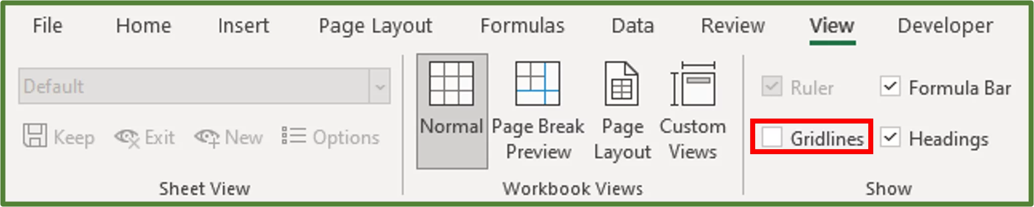
Now go to the View Tab and in the Show Group, uncheck Gridlines.
Now as soon as the student finishes a book on his reading list, he simply ticks the checkbox.
In a workplace setting, you will often have a data set that was imported into Excel from an external source. If the data looks messy you can use the trim function to quickly clean it up!
If you are struggling to make it, we have a great template here for a reading list, and a to-do list with checkboxes!
Delete Your Checkbox!
Let’s say you want to delete a checkbox you created, there are a few ways to do this.
Select the Checkbox that you would like to delete, by holding down the CTRL key and then left-clicking the checkbox.
Then simply press the delete key on your keyboard and the checkbox will be deleted.
You can also delete multiple checkboxes this way, just select them all using the CTRL key.
Troubleshooting
Let’s discuss what to do when things are not working the way you expected with your form control checkboxes.
1 – Checkbox Type
Firstly establish that it is a form control checkbox and not an ActiveX checkbox. If you right-click on the checkbox and the menu has an Edit Text option then it is a form control checkbox.
If you right-click the checkbox and the menu has a Properties option then it is an ActiveX control.
2 – Cell Links
Check your cell link box. If you drag a form control down a column, and you added a cell link to the first one:
Then all the others will be linked to that same cell.
This means you will have to change each cell link individually of each of those checkboxes.
Learning all about cell references will help you understand this concept if it sounds confusing!
3 – Size
If you find it’s difficult to see the Checkbox or work with the Checkbox because it’s too small:
Unfortunately there is no way to change the font or size of the actual square currently.
You can however use the zoom feature in Excel in the bottom right to change the size of the whole sheet!
Learning Objectives
You now know how to:
- Insert a Form Control Checkbox.
- Create a Simple To-do List Using Checkboxes.
- How to Delete your Checkbox
Conclusion
In this tutorial we have shown you how to produce a visualization by incorporating multiple checkboxes.
You can insert checkboxes to design dashboards, reports, and Excel based widgets.
Special thank you to Taryn Nefdt for collaborating on this article!


- Facebook: https://www.facebook.com/profile.php?id=100066814899655
- X (Twitter): https://twitter.com/AcuityTraining
- LinkedIn: https://www.linkedin.com/company/acuity-training/