Inserting A Check Mark (Tick ✓) Symbol in Excel

Have you ever prepared a checklist in Excel?

Checklists give you the feeling of having accomplishing a task.

Their utility comes from the check marks that you can put against different items within them.

Note: A check mark is also often reffered to as a tick mark!

Inserting A Check Mark – Copy Paste

There are several ways how you may add a check mars in Excel. But what’s easier than simply copy-pasting it?

Don’t go any further to find yourself a check mark  / tick mark – here it is.

✔

To add a check mark to any of your excel files, simply:

• Select the check mark above.
• Copy it using ‘Ctrl + C’, or Right Click it and click Copy!
• Go to the destination excel sheet and paste it into the desired cell using ‘Ctrl + V’, or Right Click and hit Paste.

Want to learn more about mathematics in Excel? Read our guide here all about Percentages in Excel.

Inserting A Check Mark – Keyboard Shortcuts

There are many variations to the appearance of a check mark that Excel has to offer.

It can be a simple tick/cross symbol or an encircled tick/cross symbol, or a tick/cross symbol enclosed in a square.

You can add a check mark to your Excel sheets simply by using some smart keyboard shortcuts.

To do so, you need to set the font style to either of the font styles listed below.

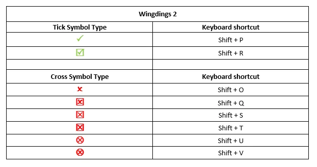
• Wingdings 2
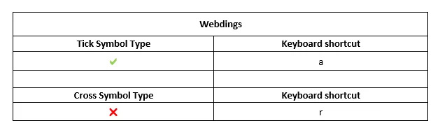
• Webdings

Each of the above font styles offers a different kind of variation to the appearance of tick/cross symbols.

The table below summarizes all the shortcuts that you need to know to add different kinds of check marks in Excel.

Wingdings 2:

Webdings:

 

Excels filter function is one of the most commonly used functions of Excel, learn about it here.

Inserting A Check Mark – Symbol Dialog Box

The built-in function offered by Excel for inserting checkmarks often goes neglected.

One of the most common ways of adding checkmarks in Excel is through the Symbol Dialogue Box.

This is a really simple tool that will make your spreadsheets more presentable.

To add a check mark in Excel using the Symbol Dialogue Box, the following steps need to be followed.

Step 1:

Activate the cell where you want the symbol inserted.

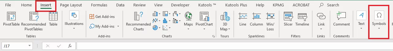
Step 2:

To insert the symbol, go to Insert Tab > Symbols > Symbols.

 

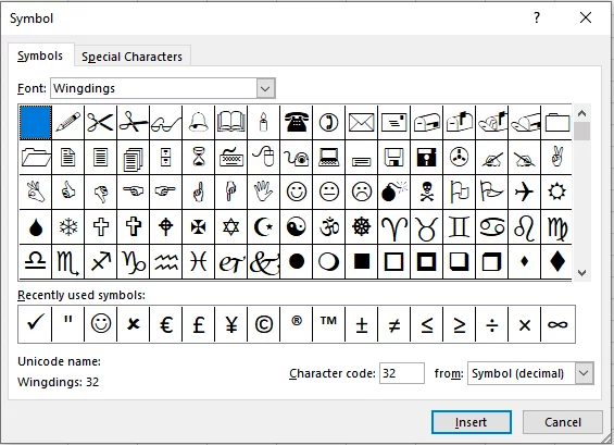
Step 3:

The Symbol Dialogue Box offers a wide variety of symbols that you can add to your Excel sheet.

However, to get each particular symbol, a specific font needs to be selected.

Tick :

To get a tick from the Symbols, select the font as ‘Segoe UI Symbol’ from the font options.

From the list of symbols that then appears, scroll to find a tick symbol.

Once found, select it and click ‘Insert’ and then ‘Close’ to have it added to your Excel sheet.

Cross :

To get a cross from the Symbols, select the font as ‘Segoe UI Symbol’ from the font options.

From the list of symbols that then appears, scroll to find a cross symbol.

Once found, select it and click ‘Insert’ and then ‘Close’ to have it added to your Excel sheet.

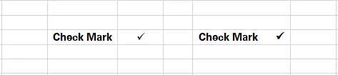
This method allows users to add checkmarks in Excel in both, an empty and an occupied cell.

It also allows users to add multiple checkmarks to a single cell.

For instance, using the method above, you can add checkmarks to both the cells as shown below.

This option may not be available with other methods that only allow adding checkmarks to an empty cell.

Note:

The font style ‘Segoe UI Symbol’ offers different styles for tick and cross-check marks.

These include simple tick mark symbols and square-enclosed tick marks.

Other styles for the same symbols can be found using different font styles, for example, Wingdings.

 

Pro Tip:

For every selected symbol, there appears a distinct character code at the right bottom of the Symbol Dialogue Box.

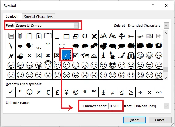
Do take note of these character codes, as they’d help you add the same symbols through a formula.

Keep calm until we learn how to do so in the later sections of this article.

Want a better view of your data? Try freezing the panes that contain headers.

Learn all about freezing panes in Excel by clicking here.

Inserting A Check Mark – Using the CHAR Function

To add checkmarks to Excel using the keyboard, in addition to keyboard shortcuts, you can also use the CHAR function.

While we discussed the use of Symbols Dialogue Box for adding checkmarks in Excel, we noted there was a character code for each symbol.

It is time to make use of this character code.

The CHAR Function

To do so, let’s learn what the CHAR function is about.

Syntax

= CHAR (number)

The number in the above formula can be any character code between 1 to 255.

Return Value

Applying the above CHAR Function, Excel returns the symbol represented by the character code.

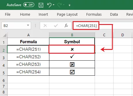
The common character codes to add a check mark in Excel are as follows.

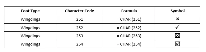
Adding checkmarks to Excel using character codes is pretty simple.

To add a checkmark, select the designated cell to activate it and enter the relevant CHAR functionto the cell.

Applying the CHAR function in Excel, the results are as follows.

Pro Tip:

This method of adding a check mark can only work with empty cells and not with cells already having values.

If you want to add a check mark to an already occupied cell, you may do it through the Symbol Dialogue Box method.

 

Inserting A Check Mark – Autocorrect

This option will suit you the best if you get to use tick marks regularly.

For instance, a teacher who often has to mark the results of his / her students and has to use plenty of check marks.

Using either of the methods above repetitively might cause you undue time and effort.

What if you set up a shortcut that will add a check mark to Excel every time and any time needed?

This can be done using the AutoCorrect function.

How can we do this? Take a look  at the Gif below to learn how!

Step 1:

The first step is to obtain a checkmark in Excel – this can be done using any of the methods explained above.

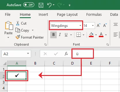
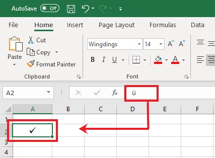
In the image above, we have added a checkmark in Excel using the Symbols Dialogue Box.

Note that the font style is set to Wingdings.

Moreover, the formula bar shows a ‘ü’ symbol.

This is the character fed into Excel, upon which when the Wingdings font is applied, Excel turns it into a tick symbol.

Step 2:

The next step is to copy this character ‘ü’ from the formula bar to set it up as an AutoCorrect Option.

Step 3:

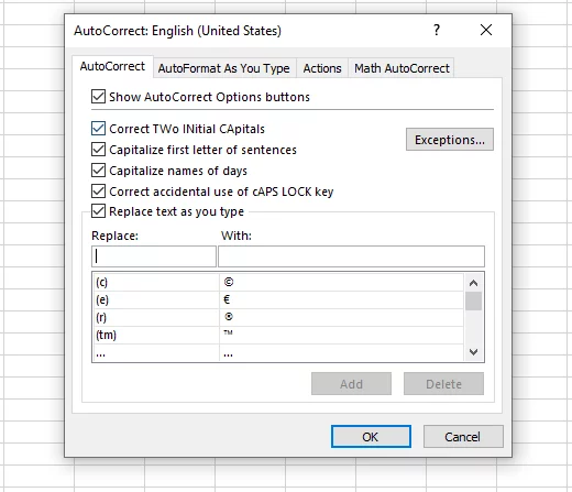
With the above-said character copied, go to File > Options > Proofing > Auto Correct Options as shown below.

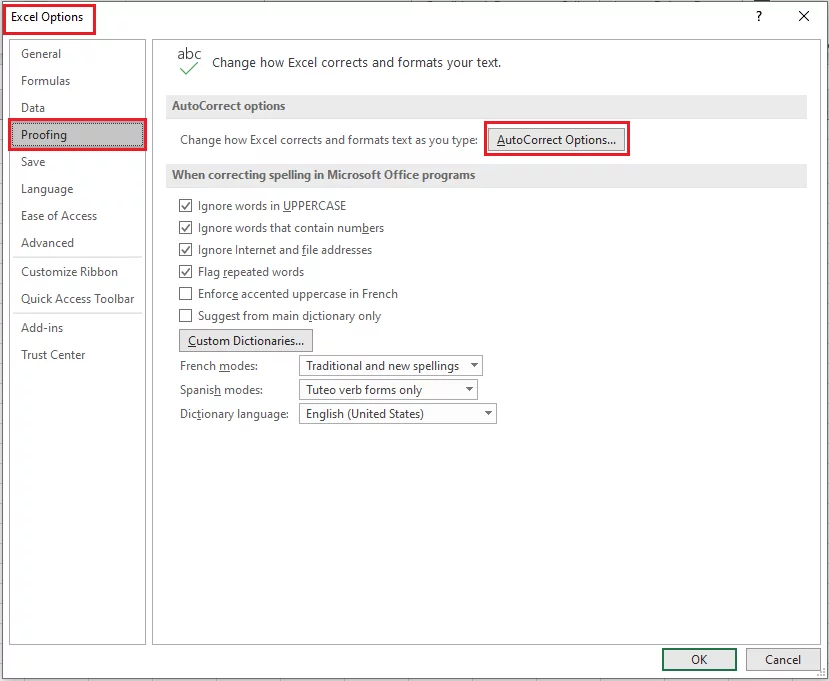
Clicking in Auto Correct will open up the AutoCorrect window as follows.

 

Step 4:

From the Auto Correct Window, populate the ‘Replace’ option with any keyword that you want replaced with a checkmark.

For instance, if you want Excel to add a checkmark to a cell every time you add a particular word to a cell.

This could be any sequence of letters or numbers.

In the example below, we have used the word ‘CMARK’ as the subject keyword.

This means, every time you input the word CMARK in Excel, it would be replaced with a check mark.

Next, populate the ‘With’ option with the symbol for the check mark that we copied in the previous step i.e. ü.

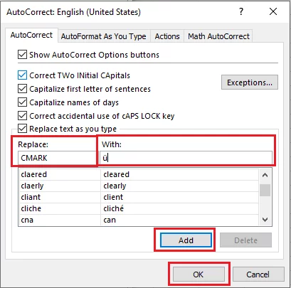
Doing so, every time you enter CMARK in any cell, Excel would replace it with an ü sign.

Once the options are set up, click ‘Add’ and ‘Okay’.

Step 5:

Technically, we are all done, and now is the show time.

To make this Auto Correct option work, go to Excel, and type the keyword set up earlier – CMARK.

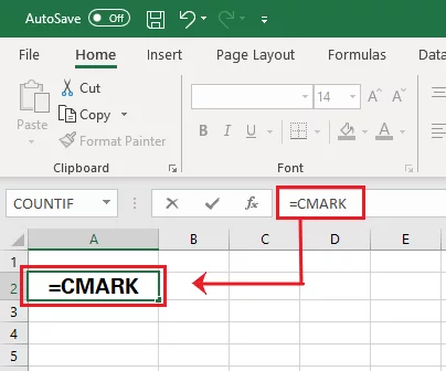
Press enter to have a tick mark entered into the cell as follows.

Inserting A Check Mark – Conditional Formatting

No end to the ways of adding checkmarks in Excel and here we have yet another one.

The conditional formatting function of Excel guides the behavior of different cells that meet a specified condition.

Using the same function, you can also conditionally add checkmarks to Excel.

Consider the data in the example below.

 

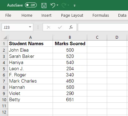
The data in the image above represents the marks of different students. Let’s assume the passing marks are 500.

Now, it might be difficult to readily visualize the data to identify students who have passed or have not passed.

To make the data easier to study, you may apply conditional formatting to it.

Under conditional formatting, all those students who have passed (i.e. scored marks more than 500) will have a tick mark adjacent to their names.

Similarly, those students who have failed may have a cross symbol adjacent to their names.

To add checkmarks to Excel using conditional formatting, follow the steps below.

Step 1:

Select the cell range where the marks are populated and go to:

Home Tab > Styles > Conditional Formatting > Manage Rule

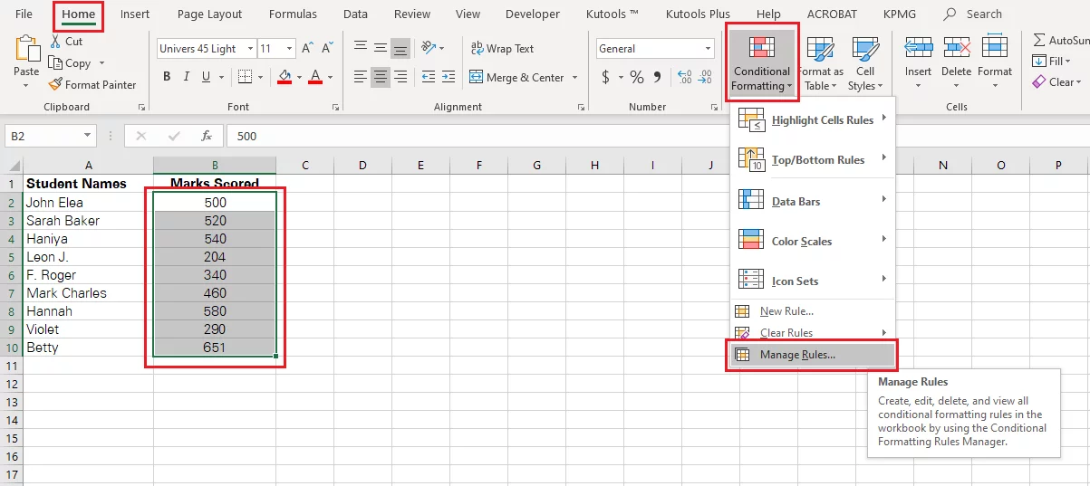
This will open up the ‘Manage Rule’ window as shown below.

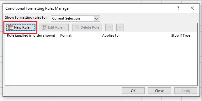
Step 2:

From the manage rule window, select ‘New Rule’ as shown above. This will open a window for you to set up a rule as shown below.

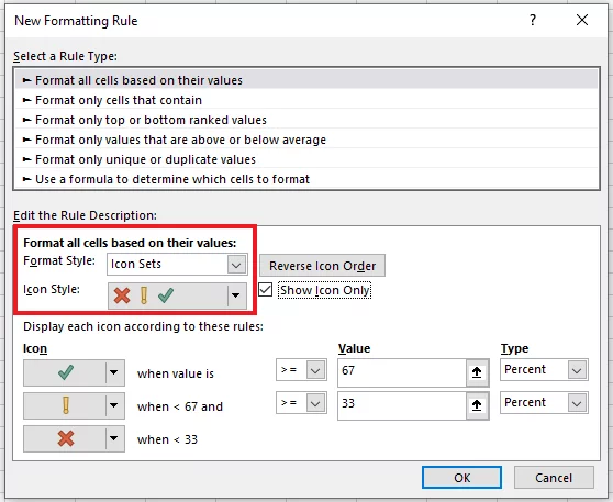
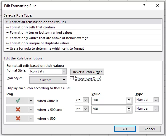
From the window above, under the Format Style, select ‘Icon Sets’.

Under Icon Style, select checkmark icons like cross, tick, and exclamation mark.

Before moving forward, select the type as ‘Number’.

This is because we will set up the rules against the value of 500.

Against the value, populate the value based on which icons are to be added. In our example, this value is 500.

 

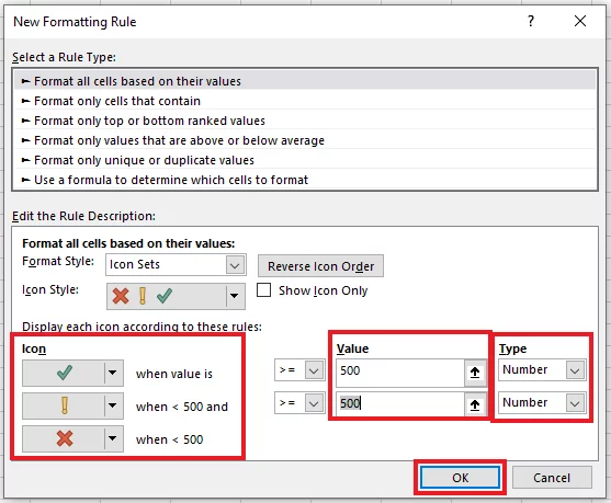
Under the Icon, select a tick icon for ‘value >’ (value more than) and a cross icon for ‘value <’ (value less than), as shown above.

For ‘value < 0’ you may select ‘No Cell Icon’

Step 3:

After the rules are set, click ‘okay’. This will add the rule to the ‘Manage Rules’ window, as shown below.

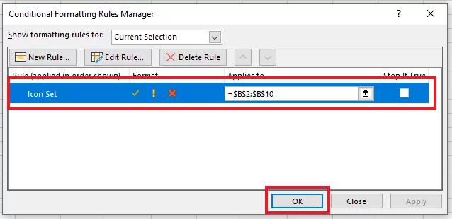
Select this rule and click ‘Okay’ to apply the rule to the selected cells.

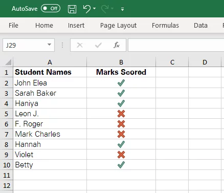
Excel will apply the rule to the selected cells, and icons will be added as shown below.

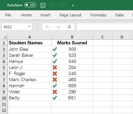
Paying close attention to the icons will make you learn that Excel has added a tick icon to all the values exceeding 500 and a cross icon adjacent to all the values less than 500.

Pro Tip:

If you do not want icons to come parallel to the values but in cells in place of the values, this can be set up in the rule as follows:

The results of checking this option are as follows:

Formatting a Check Mark

Who said a checkmark is only supposed to be a tick or cross in monochrome tones.

You can turn your checkmarks into colorful icons by exploring the formatting options offered by Excel.

There are several ways how you can format a checkmark in Excel – check out these below!

1.      Check Mark Color

There’s a general notion of positives going green and negatives going red.

Similarly, a tick mark doesn’t feel like a tick till it’s vibrant and green.

A cross mark might not be alerting enough till it’s red and sharp.

In Excel, after you’ve added a check mark, you can format them to different colors as you may like.

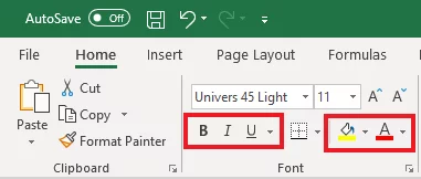
All you need to do is, select the cell containing the relevant check mark and go to:

Home Tab > Font > Font Color

From the various font color option offered by Excel, choose the desired color.

The same will be applied to the contents of the selected cell.

What if you have multiple check marks in a cell? You could apply a different font color to each check mark!

To do so, you do not have to select the entire cell containing the checkmark.

Instead, click on the cell containing the checkmarks to activate it.

Once activated go to the formula bar and select the characters for the checkmarks that you want to be colored.

With them selected, choose the desired font color from the Font tab.

Excel would change the color of the selected check mark only. Here’s a short tutorial to help you:

2.      Bolden up

To add more expression to your work, it might be important to bolden up the checkmarks.

To bolden the checkmarks in Excel, follow the steps below:

1. 1. Select the cell containing the checkmark.
   2. Go to Home Tab > Font > Bold Icon.
   3. Alternatively, select the cell containing the checkmark and press ‘Ctrl + B’

Pro Tip:

To bolden only a few check marks from a cell and not the whole contents of a cell:

Select that particular character/checkmark and press ‘Ctrl + B’.

 

3.      Other formatting options

You may opt for other formatting options to enhance the appearance of your check marks in Excel.

These options include underlining, italics, highlighting the cell containing the checkmark, or adding borders to the cell.

All of these options are readily accessible under the Font Tab from the Home Group.

Counting Check Marks in Excel

This section will be using the COUNTIF function to help count up our check marks.

If you need a refresher, click here for our guide to the COUNTIF function in Excel!

Using the COUNTIF function, counting cells that contain a specific value is very easy.

For starters, let’s say we want to count the number of 2s that appear in the below data set.

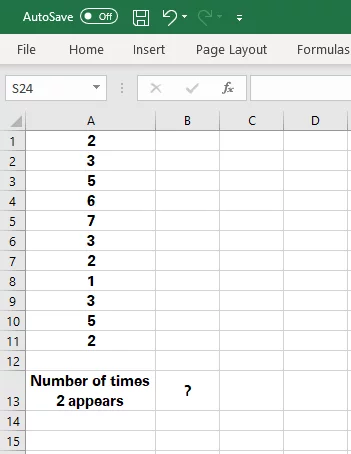
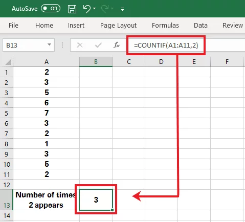
To count the number of times 2 appears in the above data set, we applied the COUNTIF function as = COUNTIF (A1:A11, 2).

Doing so, Excel yields the number of times 2 appears in the defined range of cell A1:A11 as follows.

Counting checkmarks in Excel is equally easy using the CHAR formula as the criterion. For instance, take a look at the data below.

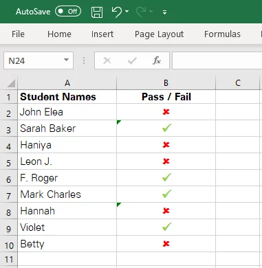
In the image above, students who have passed have a tick symbol, and those who have failed, have a cross symbol adjacent to their name.

To find out how many students have passed and how many have failed, we can apply the COUNTIF function to count the number of tick symbols and cross symbols.

But before we do that, it is important to know how we have created these checkmarks.

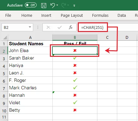
The above checkmarks are added using the CHAR formula. So, to count these checkmarks, the COUNTIF formula will be set up as follows.

To count tick marks:

= COUNTIF(B2:B10, CHAR (252))

To count cross marks:

= COUNTIF(B2:B10, CHAR (251))

The first argument i.e. B2:B10 is set as it represents the range where the checkmarks are placed.

Time to see the COUNTIF function in action:

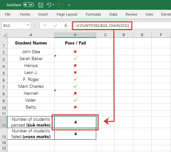
Excel has counted the tick marks in the data to be 4 using the COUNTIF Function.

This ultimately means that 4 out of the total students have passed.

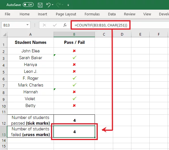
Excel has counted the cross marks in the data to be 4 using the COUNTIF Function.

This ultimately means that 4 out of the total students have failed.

Here is a quick tutorial on how you can count check marks in Excel using the COUNTIF function.

 

Pro Tip:

Counting check marks in Excel is super easy and straightforward.

However, the method above has a few limitations that you must bear in mind.

The COUNTIF function will only enable check mark counting for a check mark that has a specific character code.

Troubleshooting

Without a doubt, adding checkmarks in Excel is a child’s play.

However, even then there are chances of things not going as expected.

If you are facing issues with inserting a check mark in Excel, check for the following issues:

Inappropriate Font

After we have discussed several methods of adding a check mark in Excel, you know how important the font type is to get the desired check mark in Excel.

For instance, if you are inputting = CHAR (252) and instead of a tick mark, Excel returns the character ‘ü’, you are probably going wrong with the font type.

To fix the said issue, select the relevant cell and change the font type to ‘Wingdings’.

 

Vacant Cells

Some methods of inserting a check mark in Excel like the CHAR formula, and the Autocorrect option will not work if you already have some data in the destination cell.

If you want to add a check mark to a cell alongside some other data, the appropriate method is of the Symbol Dialogue box or copy-pasting in the formula bar. Take a look below.

Conclusion

Now you know everything about making check marks in Excel.

These are a great tool for making your data more approachable and satisfying.

You can bring the information to use in several ways, for example in reports, result cards, forecasts, financials, etc.

For more on Excel, check out our Using AI With Excel article here!