
Ultimate Guide: Highlighting Duplicate Values Excel
Contents
In the working world, data is never perfect and needs cleaning up before you analyse it.
If you’ve ever been handed a big data set for analysis, you’ll know they come full of duplicate values!
This means it’s crucial to remove duplicates for data analysis to work.
Many delegates on our London Excel training courses find this to be one of the most valuable topics to master.
How To Highlight Individual Values
Let’s take a look into how the Highlight Duplicates in Excel function works, which is essential for highlighting duplicates effectively.
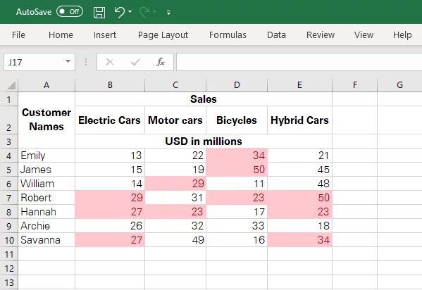
Beginning with a simple example, below is an image that represents a table of invoices arranged customer-wise.
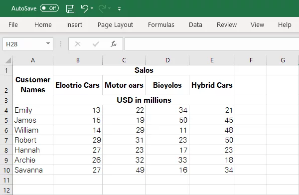
It shows the amount invoiced to each customer against the purchase of different modeled cars.
Within this data set, you may want to highlight duplicate values to easily identify and manage duplicate entries.
- All purchases of the same value within either of the models (categories).
- All purchases of the same value within each of the models (categories).
Highlighting Duplicate Values From Multiple Rows:
To effectively manage your Excel sheets, it’s important to know how to highlight duplicate rows, ensuring that you can highlight duplicate entries with precision.
To filter out all purchases of the same value within either of the models (categories), here are the steps to follow.
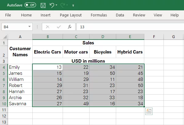
Step 1: Select the data range from where you want to pick out duplicate values.
In the given example, as we want to select purchases of the same value from all the models, the entire dataset containing numbers is selected.
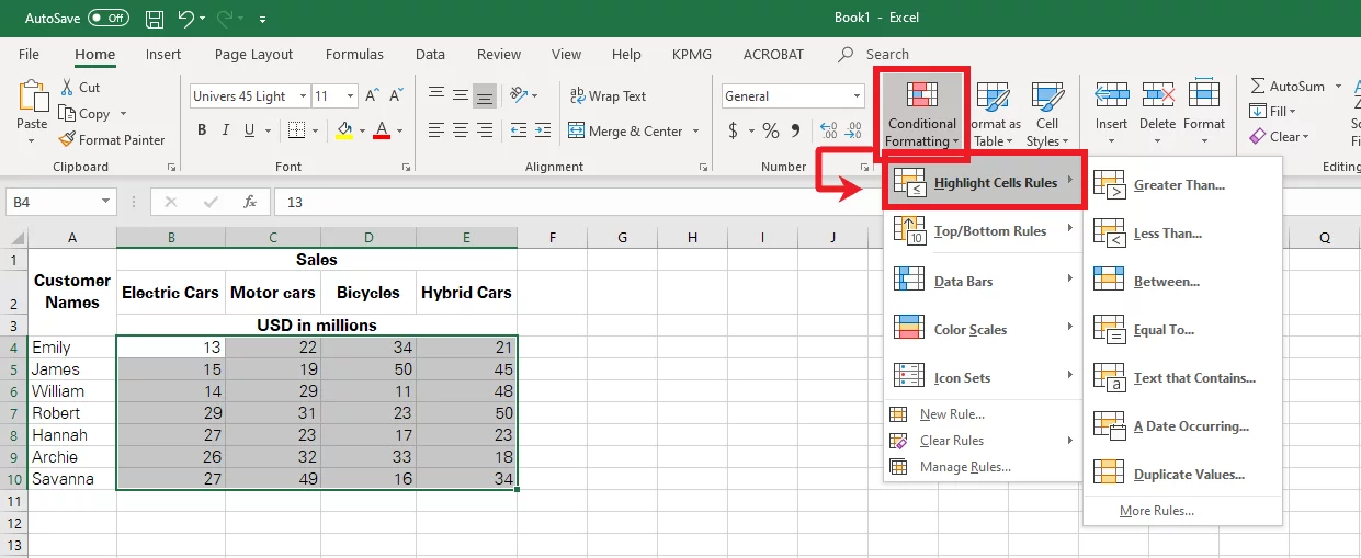
Step 2: With the data range selected, go home, go to the ‘Styles’ tab, tap on the ‘Conditional Formatting’ section to see a drop-down menu of options as follows.
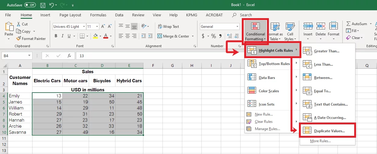
Step 3: To select the duplicate values from the dropdown menu of Conditional Formatting, select ‘Highlight Values’ and then select ‘Duplicate Values’ as shown in the screenshot below.
Step 4: Choosing this option would open a Dialogue box as evident from the screenshot below.
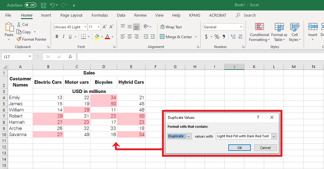
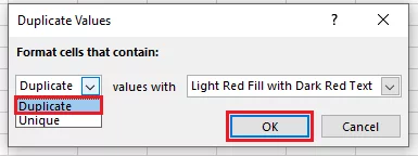
The dialogue box, as above, presents you with two choices to make. From the first option, you must select the ‘Duplicate’ option.
From the second dropdown menu, you can choose any formatting that you may want to be applied to the duplicate values.
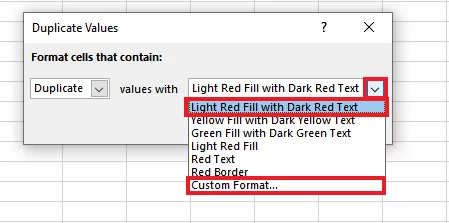
Excel presents you with the most commonly chosen options by most excel users.
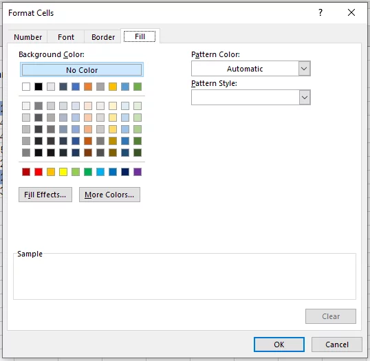
However, if you want different formatting to be applied to, you can choose the ‘Custom’ formatting option as below and custom the formatting to your choice.
This allows you to choose between various format settings including the Font style, the border style, and the fill style.
Mastering Excel’s font formatting tools really helps when presenting your data.
Once you have applied the function, excel highlights duplicates for you from the entire selected range of cells.
All of the highlighted cells indicate values that have occurred two or more times in the entire selected range.
Highlighting Duplicate Values From Individual Rows / Columns:
Understanding how to highlight duplicates in Excel rows / columns is very important, especially when dealing with duplicate cells in your datasets.
Lets say you want to filter out invoices of the same value within every single model of car.
For example, you may want to identify invoices of the same value from the Electric Cars only.
To filter out all purchases of the same value within each of the models (categories), here are the easy steps that you need to follow.
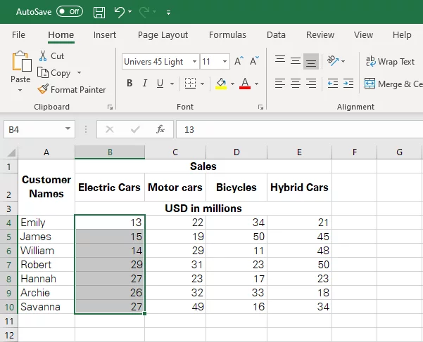
Step 1: Select the data range (the single row/column) from where you want to pick out duplicate values.
In the given example, as we want to highlight duplicates within Electric Cars only, the column containing invoices of Electric Cars (i.e. Column B) is selected only.
Step 2: With the column selected, go home, go to the ‘Styles’ tab, tap on the ‘Conditional Formatting’ section to see a drop-down menu of options.
To select the duplicate values, from the dropdown menu of Conditional Formatting, select Highlight Values and then select Duplicate Values.
Choose the formatting you’d want to apply to the duplicate values, and you are done.
Excel would highlight the duplicate values for you within a single column as follows:
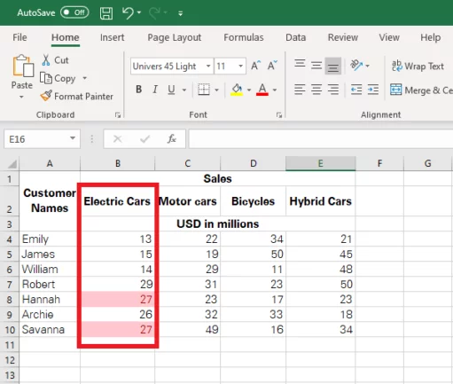
Now you can go through and find the important data. This is a great method to save you time doing manual work in spreadsheets.
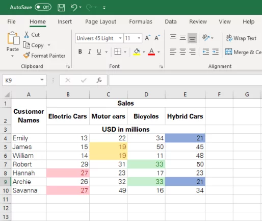
You may also highlight duplicate values within each column separately.
For example, to identify and highlight duplicate values appearing within each individual model of cars:
You may repeat the above process for every single column, and excel would highlight duplicate values from each column as follows.
Another way to highlight duplicates is using conditional formatting, which you can set up in advance!
What Is The COUNTIF Formula?
The COUNTIF function counts the number of cells appearing within a defined range that meets a specified criterion.
However, this function is also used to highlight duplicate values within excel.
It outstands the contemporary ‘Conditional Formatting’ function as it allows defining commands of your choice.
Unlike the conditional formatting rule whereby you can only command excel to pick out duplicates.
Syntax:
= COUNTIF (range, criteria)
Within the above syntax, range defines the range of cells whereupon the COUNTIF formula is to be applied, whereas criteria defines the criteria to be applied to identify duplicate values.
How can you use the COUNTIF Function to highlight duplicates within excel?
Using the COUNTIF function to highlight duplicates or triplicates in Excel helps in efficiently managing duplicate data.
1: Select the range of cells, reach out for the ‘Conditional Formatting’ function in the ‘Style’ section of the ‘Home’ tab and select ‘New Rule’.
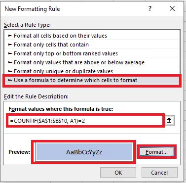
2: Choose the option ‘Use a formula to determine which cells to format’.
3: Feed in the formula using the above syntax. Define the range of cells and then specify a condition. For example, you may customize the COUNTIF formula as follows:
=COUNTIF($A$1:$B$9, A1)=2
The absolute reference ($A$1:$B$9) defines the range A1:B9 for excel, whereas the argument A1 defines the criterion for cell identification.
Excel will identify and highlight cells that contain the same value as that in cell A1 and the same formula is automatically amended and applied to all the cells within the selected range.
If in the defined range i.e. A1:B9, any value appears for 2 times, excel will identify and highlight those cells as in the screenshot.
Once you have specified the formula, make sure to set up a formatting style that you’d want to be applied to the highlighted values as can be seen in the screenshot below.
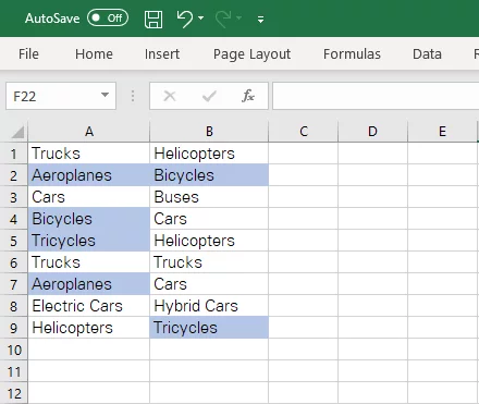
And that is how it works. Excel has highlighted all the cells that contain duplicate values only.
What you must note here is that excel has not highlighted values that appear more than twice like ‘Trucks’ & ‘Cars’.
You can therefore amend the COUNTIF Formula to yield results of your choice.
For example, you may amend the foregoing formula as =COUNTIF($A$1:$B$9, A1) = 3 and excel would highlight all triplicate values as follows.
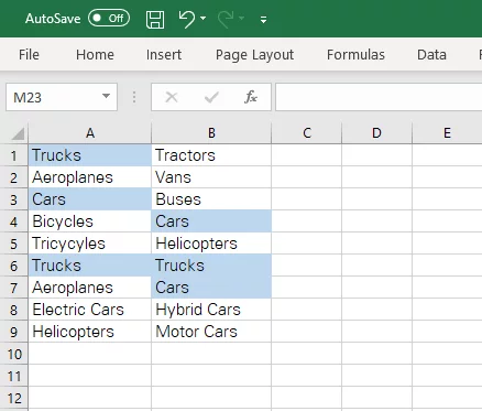
Excel has now only highlighted the triplicate values from the data range i.e. Trucks and Cars, and not the duplicate values.
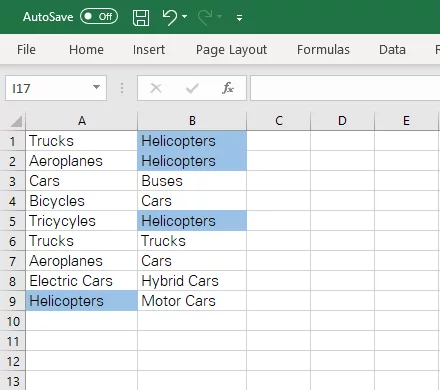
You may also amend the formula as =COUNTIF($A$1:$B$9, A1) > 3 to yield results where excel would highlight all values that appear more than 3 times in the given data set.
For example, in the screenshot below, excel has highlighted only those values that appear for more than thrice i.e. Helicopters.
Note: While writing up a COUNTIF Formula, always define the upper left value as the criterion.
Excel will automatically fill in the series and copy-paste it to the rest of the cells as
=COUNTIF($A$1:$B$9, A2)=2 in A2, =COUNTIF($A$1:$B$9, B2)=2 in B2 and so on.
Also, if the above formulas are a little too complex to remember or compose, you may give a descriptive name to your cell range and use the same while defining the above formula. Read more about named ranges in excel here.
How To Highlight Rows In Excel
The illustrations demonstrated above explain how you may highlight duplicate values within excel at the cell level.
But can Excel highlight a whole row based on duplicate values in one specific column, multiple columns, or all columns?
This is where understanding how to highlight duplicate rows becomes essential.
The built-in preset of excel for highlighting duplicate values through Conditional Formatting > Highlight Values > Duplicate values only works when at the cell level.
If you want to highlight an entire row based on duplicate values appearing in any one or more columns of that row, you’ll have to employ the COUNTIFS function as follows.
COUNTIFS
The COUNTIFS function is particularly useful when you need to highlight duplicates in Excel across multiple columns, making it easier to identify duplicate rows.
Or, by contrary, rows that have the same values in multiple columns.
Employing the COUNTIFS function helps you compare, evaluate and identify data against multiple criteria in contrast to the COUNTIF function where you can only define a single criterion.
For example, if you have a data set that constitutes multiple columns, go to Conditional Formatting > New Rule > Use a formula to determine which cells to format and write the COUNTIFS formula as follows.
= COUNTIFS ($A$2:$A$10, $A2, $B$2:$B$10, $B2) = 2
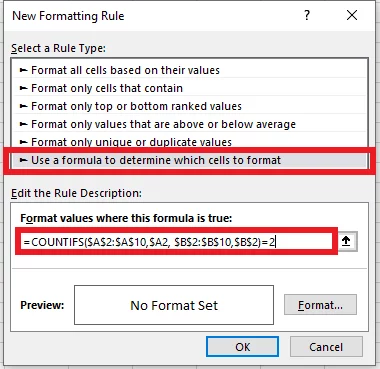
Excel would yield results as follows.
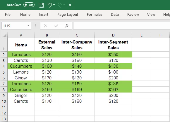
It is important to note how excel has highlighted all those rows that constitute duplicate values in Column A & B.
Row 7 and 8 constitute the same values in Column A & B as that of Row 1 and 4.
However, despite containing the same values in Column A (Ginger and Carrots), row 9 and 10 were not highlighted by excel as they contained different values in column B.
Using the COUNTIFS function, excel evaluates data against each defined criterion and only those rows that meet all the criteria are highlighted by excel.
Note: The COUNTIFS function works exactly like the COUNTIF function.
You can amend the COUNIFS formula to identify triplicates by substituting the ‘2’ in the above formula with ‘3’. Or you may set criteria as ‘>1’ or ‘<3’ etc. You can also add define additional criteria to the above formula. For example,
= COUNTIFS ($A$2:$A$10, $A2, $B$2:$B$10, $B2, $C$2:$C$10, $C2) = 2
Highlighting Duplicates: Use Cases
The smart duplicate identification function of Excel can come in handy for several reasons, such as when you need to highlight duplicate cells or highlighting duplicate values across your data sets.
While the uses may be endless, this function is commonly used for the following purposes:
- Compilation of academic results
- Sophistication of large sets of data
- Data sampling for audit
- Preparation of accounts
- Preparation of bank reconciliation statements
Once you apply the function to a given range of data, excel identifies the duplicate values as per the defined criteria and highlights them for users as follows.
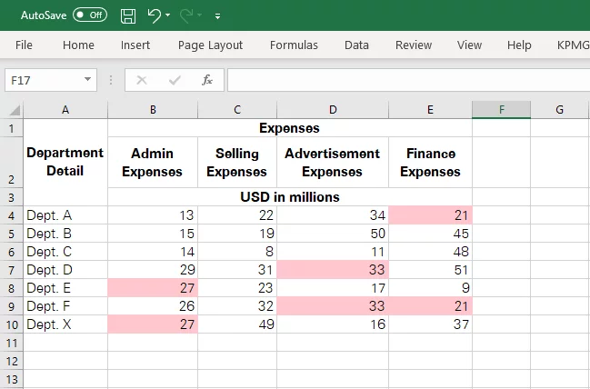
You may command excel to highlight for you a single cell or a whole row that constitutes duplicate values.
Once the dupes are identified, you can remove them, segregate or aggregate them or work them out just as you like.
Troubleshooting
Some common problems that users face while using the above-explained functions are as follows.
1. Formula Errors
If you use the COUNTIF formula, the accuracy of results are always going to depend on the formula you define.
Auditing your formulas for accuracywill help.
Also, the COUNTIF formula requires you to define a condition, which if it turns out to be true:
The formula will be triggered and excel would accordingly identify and highlight figures.
The condition you define must meet your demands.
For instance, if you define a formula as =COUNTIF($A$1:$A$10, A2)=2, excel will only highlight values that appear twice.
However, if you define the COUNTIF formula as =COUNTIF($A$1:$A$10, A2)>1, excel will highlight all those values that appear more than once (i.e. all duplicates, triplicates, and values that appear for more than thrice).
2. Excel Not Recognizing Duplicates
It is often the case that you see a value appearing twice in the given data but, the same is not highlighted by excel.
This is often the case when you have not selected the entire data range!
3. Long Strings
Although highly unlikely, but if your data set consists of cells that contain values exceeding 255 characters:
The COUNTIF function might return incorrect results when used to match such lengthy strings.
4. Case Of Characters
Neither the simple conditional formatting rule nor the COUNTIF function of excel is considerate of cases of the values.
For example, if your selected cell range consists of ‘Apple’ in cell A1 and ‘apple’ in cell A2:
Excel would highlight them both irrespective of the cases of characters being different in both the words.
5. Wildcard Characters
When using wildcard characters like a question mark [?] in any of the values appearing in your data set be careful!
A question mark matches any character in its place, be it a special character, a number, or an alphabet.
For example, if cell A1 contains ‘Apple?’ and cell B1 contains ‘Apple.’ Or ‘Apple1’ or ‘Apple!’, excel will highlight them.
Here excel matches the question mark with every character in its place, [.], [1], [!], or any other character.
Conclusion
If you are a regular excel user or even if you use excel rarely, you’ll surely come across the need to identify unique or duplicate values appearing in your data.
And when dealing with a large volume of data, it can often get super hectic to pick out duplicate values.
Highlighting duplicate values using the smart functions of excel is child’s play, and if you put in some effort, you will likely master it soon.


- Facebook: https://www.facebook.com/profile.php?id=100066814899655
- X (Twitter): https://twitter.com/AcuityTraining
- LinkedIn: https://www.linkedin.com/company/acuity-training/