
3 Quick And Easy Ways To Make Named Ranges
Contents
How would your data look if it had clear written descriptions instead of generic titles?
It would be easier to present, and for others to work with.
Named ranges are one of the most underrated features of Excel.
A named range is a descriptive name given to a single cell or range of cells.
Many people on our Excel courses in London and online even say they have never heard of named ranges!
Method 1 – Define Name
In the example below, we have a data range in Excel that shows common beverages.
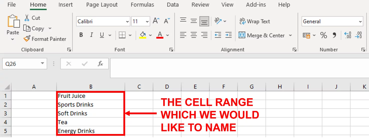
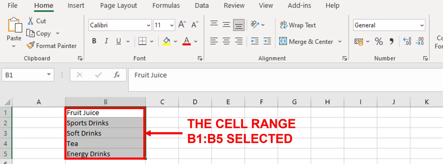
1. Select the cell range B1:B5, which contains the data.
2. With the range selected, go to Formulas on the ribbon, and in the Defined Names group, choose Define Name.

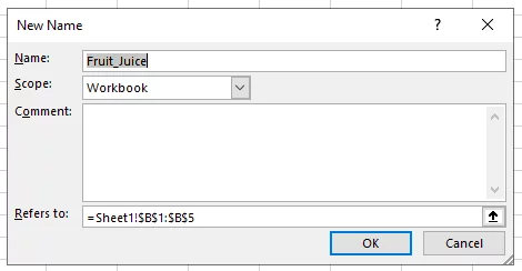
3. The New Name box will appear.
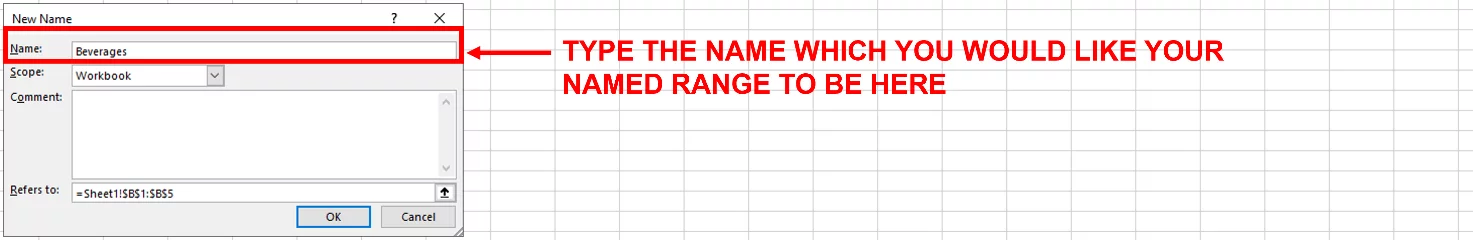
4. Using the New Name box:
Type the name which you’d like your range to be. In this case, “Beverages”.
The Scope refers to where the named ranges can be applied.
The default setting is the workbook, which means that you can use the named range anywhere in the workbook.
In this case, we will leave the default option.
If the scope is set to worksheet, then the name will only be recognised in the worksheet.
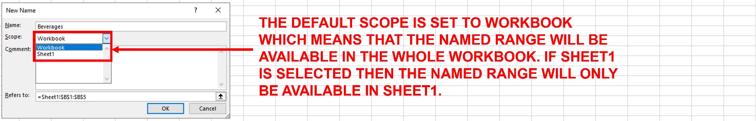
You can add a comment to provide more information about the range.
In Refers to: check that the range of interest is selected.
By default, Excel makes this an absolute reference, meaning this data will stay static no matter what.
5. Click OK.
Method 2 – The Name Box
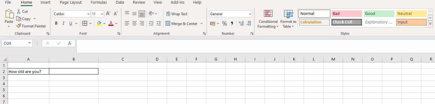
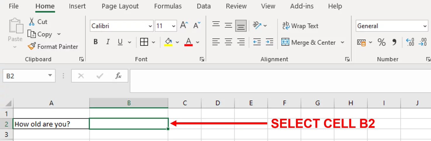
In the example below, we have cell B2, that will contain the age of the user.
1. Select cell B2.
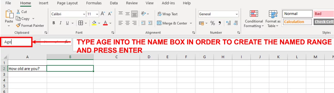
2. Using the Name Box, type Age and press Enter.
3. If you click on the Name Box drop-down arrow, you will see the named range.
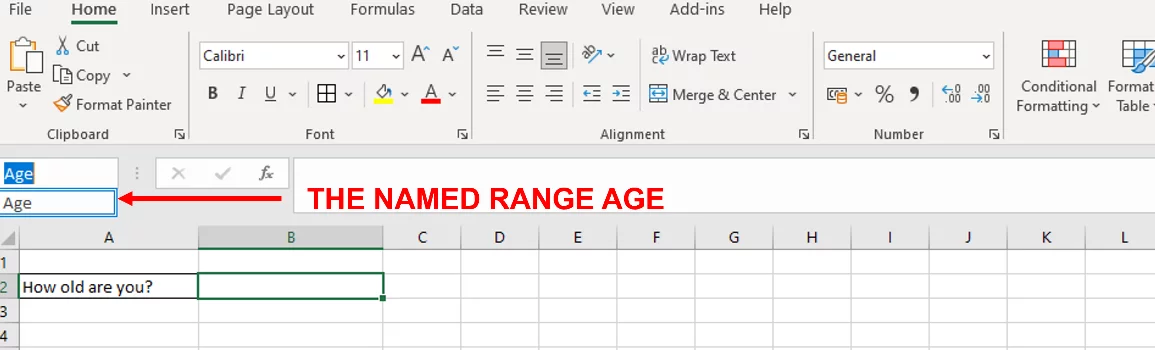
4. If you click on the named range, then cell B2 will be selected.
Method 3 – Name Manager
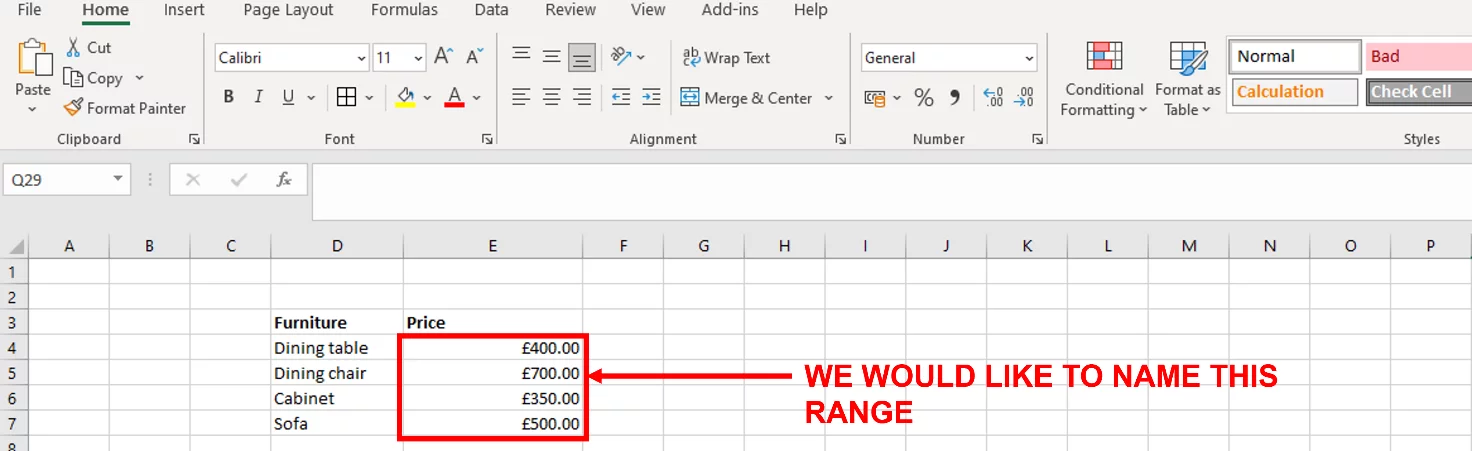
In the example below, we have a list showing an item of furniture and its corresponding price.
We would like to name the range containing the prices.
1. Go to Formulas (Step 1 in the image) on the ribbon and on the Defined Names group, choose Name Manager (Step 2 in the image).
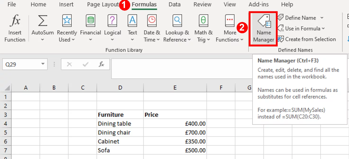
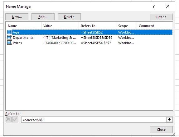
2. The Name Manager window should appear.
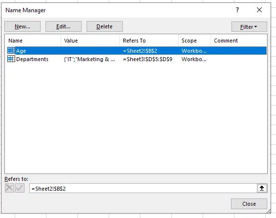
3. Click on the New button…
The New Name window should appear.
4. Enter a name for the range, which in this case is Prices. Select the range E4:E7 in the Refers to: section.
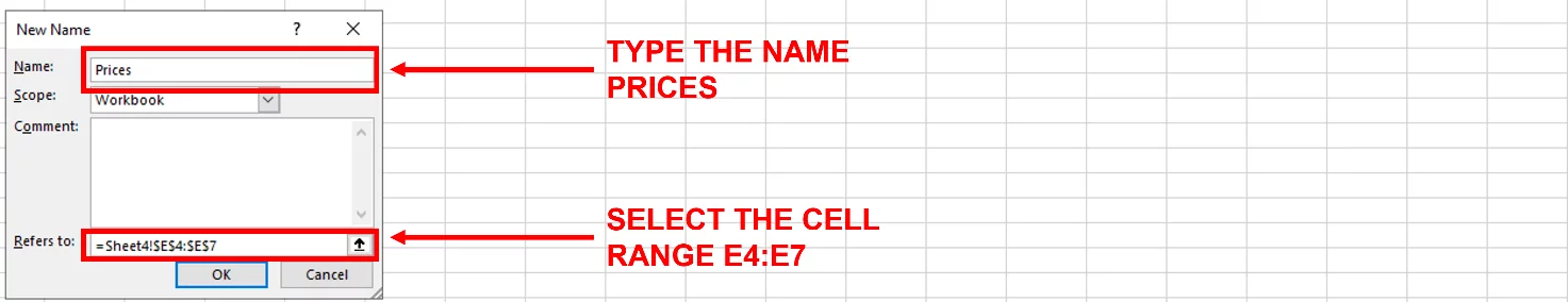
5. Click OK.
6. You should now have a named range called Prices.
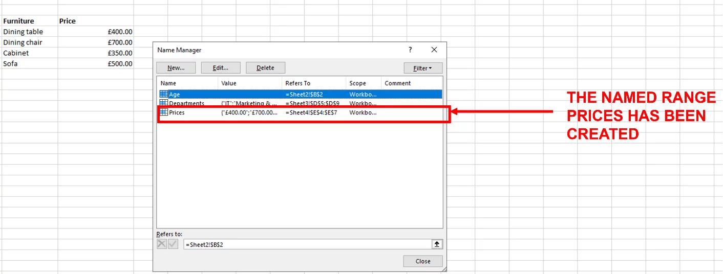
7. Click Close.
Having a Named Range makes it much easier to understand and analyse your data, as it adds more clarity to what you are looking at!
Names Ranges And Formulas
Named Ranges can even be used with formulas!
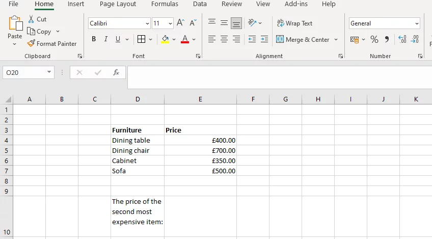
To illustrate this, let’s use our example above, where we named our Prices range.
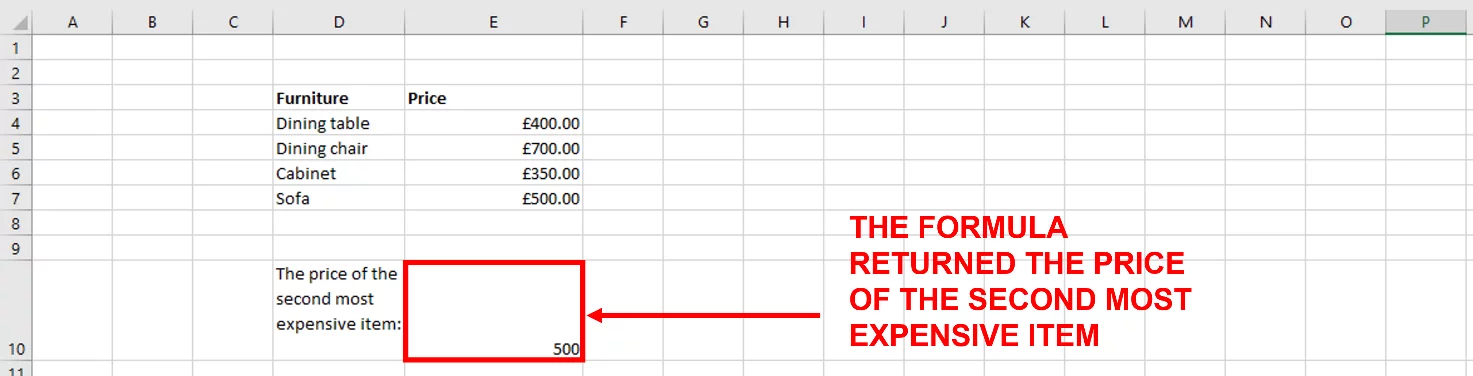
We want to find the price of the second most expensive furniture item in cell E10.
To do this, we are going to use the LARGE Function in combination with our named ranges.
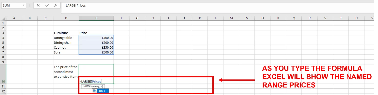
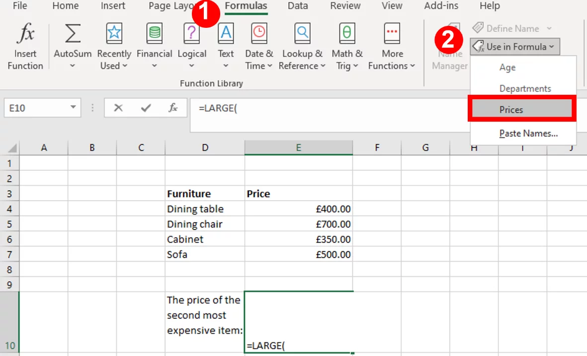
1. Select cell E10 and type the following formula using our named range Prices.
As you type Prices, Excel will show a drop-down displaying the matched name.
2. Press Enter.
3. The second most expensive value is returned.
Tip: Alternatively, you can also select the cell or cell references of interest.
Then enter the equals sign and LARGE. After opening the parenthesis go to Formulas (Step 1 in the image) on the ribbon and on the Defined Names group, click on Use In Formula (Step 2 in the image) and select the name of the range.
Complete the rest of the formula and press Enter to get the second most expensive item.
Editing A Named Range
You can edit or change named ranges in Excel by using the Name Manager.
We would like to edit the Price’s named range, which we created in the example above.
To edit named ranges, do the following:
1. Go to the Formulas Tab on the ribbon and on the Defined Names group, choose Name Manager.
2. The Name Manage window will appear, which should show you all the named ranges you have created and any tables that you may have in the workbook.
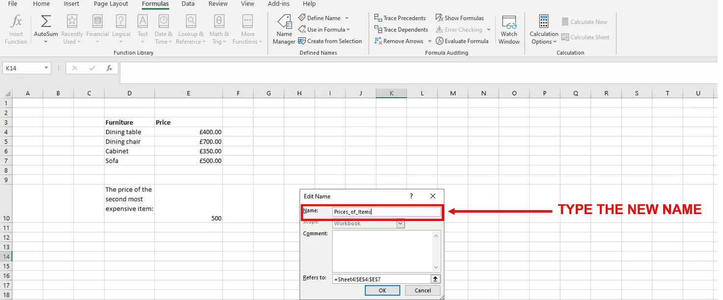
3. Select the Prices named range and click on the Edit… button.
4. The Edit Name window should appear. We would like to change the name of our range to Prices_of_Items, so type this into the Name section.
5. Click Ok.
6. Close the window.
Deleting A Named Range
You can delete named ranges by using Name Manager.
1. Go to the Formulas Tab on the ribbon and on the Defined Names group, choose Name Manager.
2. Select the named range that you would like to delete, in this case it is Departments and click on the Delete button.
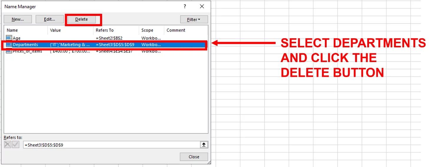
3. Click Ok to confirm and this named range should now be deleted.
Creating a Dynamic Named Range
A dynamic range refers to a range that updates automatically as new values are added to the source data.
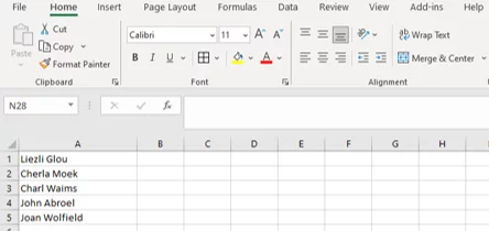
Let’s say we have a worksheet containing the names of potential contestants in column A. We want to create a range, and have it update automatically as we receive applications.
The source data is shown below.
1. To create a dynamic named range. Press Ctrl-F3 to open the Name Manager.
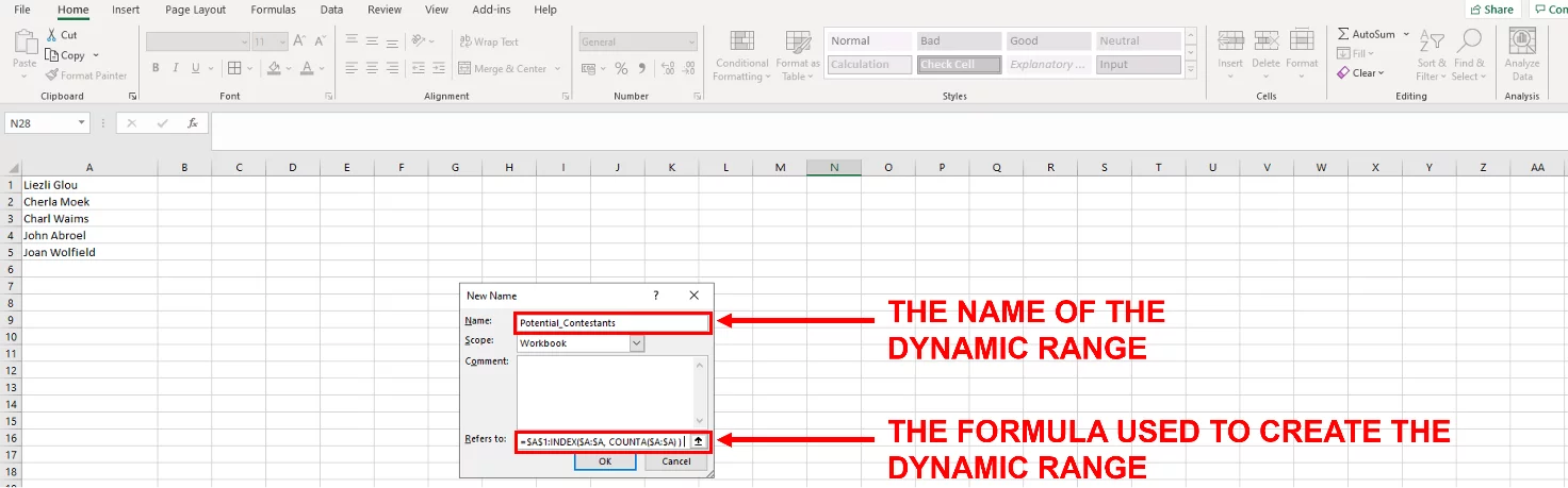
2. Click the New button…
3. Name the range Potential_Contestants.
In the Refers to: section enter the following formula:
=$A$1:INDEX($A:$A, COUNTA($A:$A) )
4. Click Ok and Close.
The INDEX Function is being used to return the reference of the last cell that has data in column A.
Since the starting point was given as $A$1 the entire formula will return the range starting from A1 to the last used cell.
It was ideal in this situation, but there are other lookup function! Knowing when to use INDEX vs Vlookup will keep your data matching efficient.
Why Use Named Ranges?
The advantages of using named ranges include:
-
You don’t have to physically select the cell range each time you want to use it.
-
You don’t have to remember the cell references.
-
Named ranges can be managed easily by using Name Manager.
-
Navigation to named ranges is much easier through the Name Box feature.
Useful Shortcuts
Ctrl+F3 opens the Name Manager’s Window.
Ctrl+Shift+F3 opens the Create Name from Selection Window.
These keyboard shortcuts perform the same operations, just much quicker!
Conclusion
You can see the benefits of using an Excel named range in your workbooks.
Named ranges in Excel make your formulas easier to understand.
You can name Excel lists to simplify your workbooks.
Special thank you to Taryn Nefdt for collaborating on this article!


- Facebook: https://www.facebook.com/profile.php?id=100066814899655
- X (Twitter): https://twitter.com/AcuityTraining
- LinkedIn: https://www.linkedin.com/company/acuity-training/