Calculate Percentage Difference in Excel [2 Practical Examples]

In this post, we will review how to calculate the Percentage Difference in Excel.

Percentage Difference is the absolute value change of two values, divided by the average of them.

The result is then multiplied by 100.

Excel has a number of ways you can represent a percentage, and work them out!

This article will cover everything you need to know to calculate a Percentage Difference using Excel.

Want to learn more about Excels most valuable formulas and functions?

Percentages are used in every industry, so delegates are always asking about this topic on our MS Excel courses.

Calculating The Percentage In Excel

We’ll start with the basics and look at how to calculate percentage in Excel. Just a reminder: percent means a part of 100.

In our example, we have data from a hypothetical e-commerce store. The owner of this store checks how many of their daily visitors sign up for news about sales and promotions.

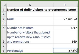
The source data for the date of interest is shown below:

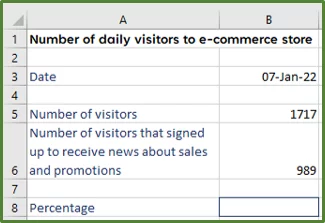
We want to calculate the percentage of people that signed up to receive sales and promotional news out of the total daily visitors, which is 1717.

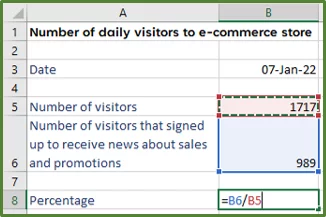
1)   So, to do this in cell B8, enter the following formula:

=B6/B5

2)  Press Enter, and you should see the following.

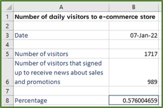
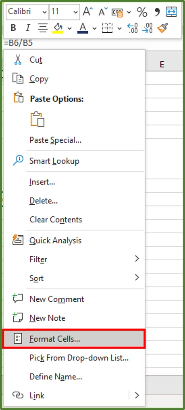
3)   Now right click cell B8 and choose Format Cells…

4)   Now, using the Format Cells Dialog Box, select Percentage and enter 1 decimal place.

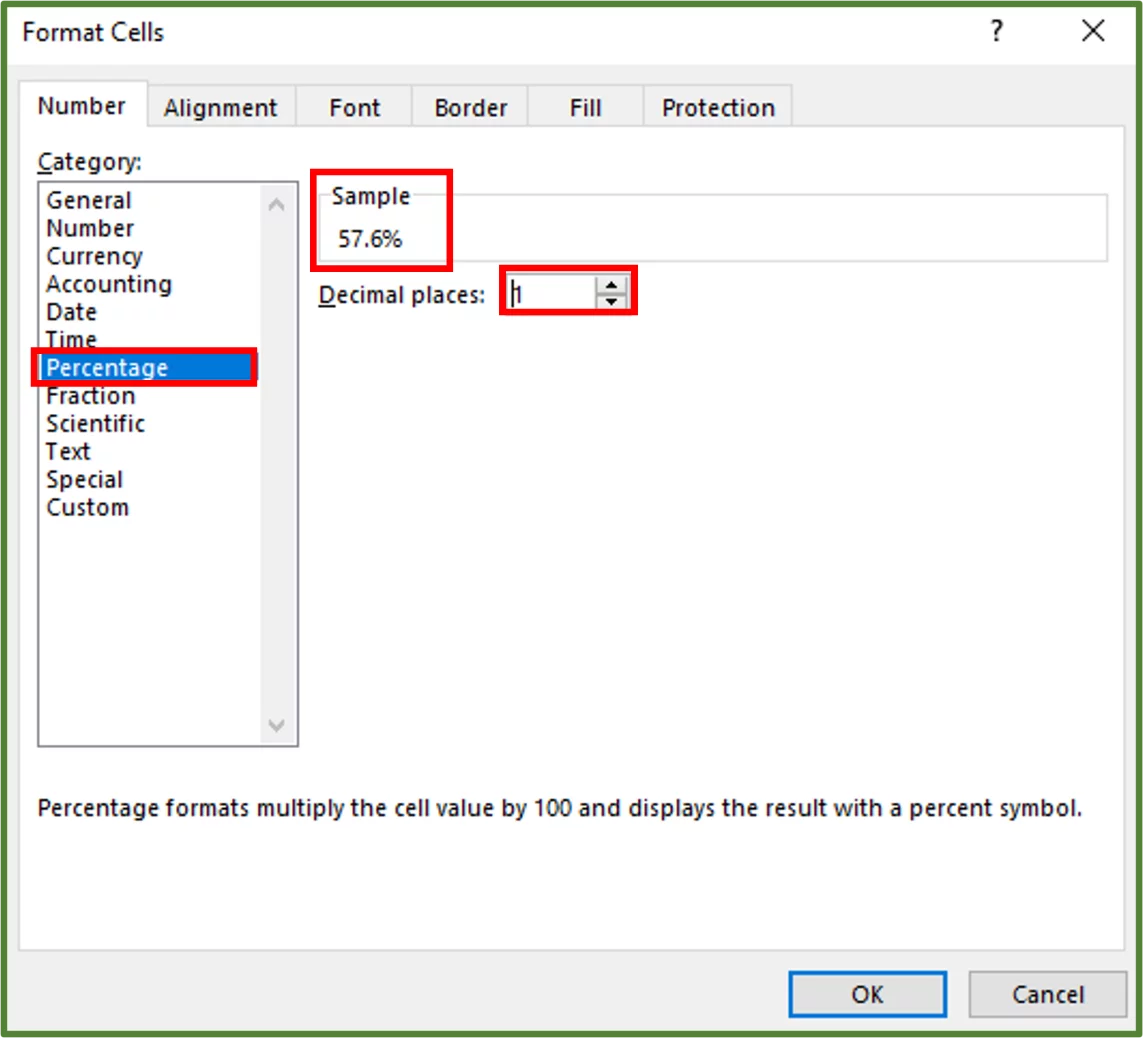
5)   Click Ok.

 

When Excel applies percentage formatting, it multiplies the value in the cell of interest by 100.

We find on our courses this is the most important step to understanding Excel percentage difference.

Once data is put into a percentage format it can be very useful to model it correctly.

Read our guide here on Stacked Bar and Column Charts.

Displaying Numbers As Percentages In Excel

You need to remember a few things when you are calculate percentages in your workbooks.

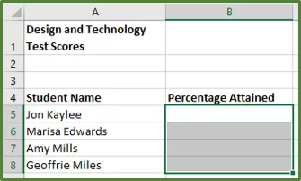
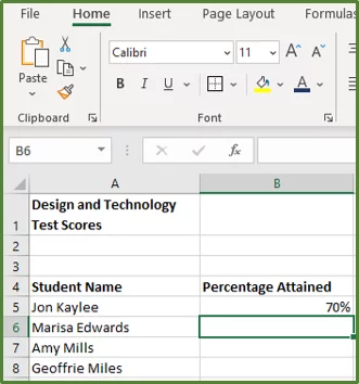
Let’s say we want to record some students’ hypothetical Design and Technology test scores.

We enter the student name in one column and the percentage they received in another column.

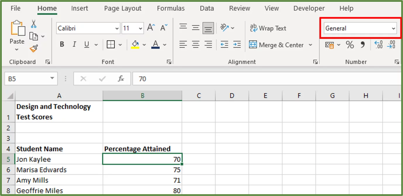
We can see that the General format gets applied by default. We want to display the numbers in column B as percentages.

If we select cells B5:B8 and went to the Number Group on the Home Tab and chose %. We would get the following.

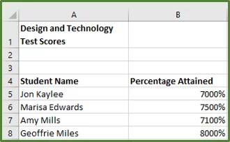
Since we applied the percentage format to numbers that we had already entered into our worksheet Excel multiplied each value by 100 to convert to percentage.

One way to fix this would be to enter the numbers as decimals before changing the formatting.

So, in cell B5, for example, if we entered 0.7 instead of 70 and then applied the percentage format, it would display correctly.

Another way to do this is, before we enter the numbers, to select the range B5:B8.

With this range selected, go to the Home Tab (step 1 in the image) and on the Number Group, choose Percent (step 2 in the image).

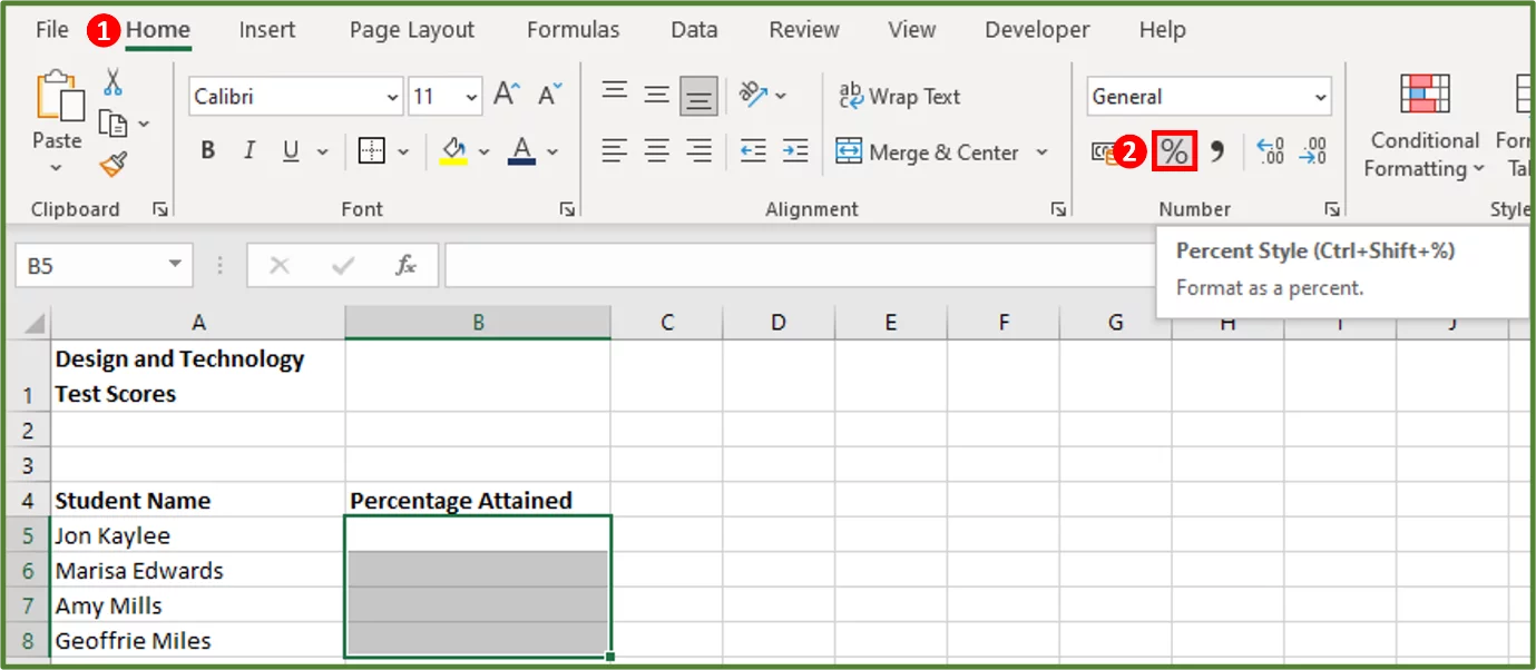
You should see that the format has been applied to the select range.

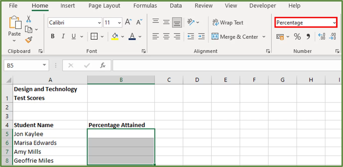
Now, if we type 70 in cell B5, for example, we will get the following.

As a valuable form of finding information, working out percentage differences feeds into helping a user Analyse Data in Excel.

Excel Percentage Difference Details

The percentage difference calculation looks at the absolute difference between two values divided by the average of the two values.

This value needs to be displayed as a percentage.

Both values should be the same type of thing. For example, comparing the heights of two houses or the lengths of two sheets of paper. Neither value should be more important or have a higher weighting than the other.

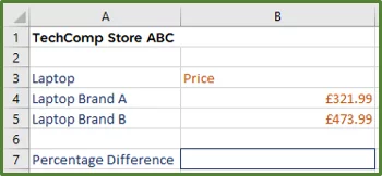
Let’s look at a simple example, we have a hypothetical store selling laptops and other IT equipment.

We will look at the percentage difference between the prices of two of the laptop brands.

1)   So, in cell B7, we type the following formula:

=(B5-B4/AVERAGE(B4:B5)

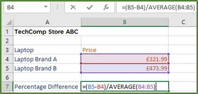
2)   Press Enter.

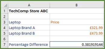
3)   Now, with cell B7 selected, go to the Number Group on the Home Tab and apply Percentage formatting. Note: You can increase or decrease the number of decimal places as required.

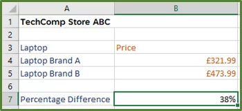
The percentage difference between the two values is 38%.

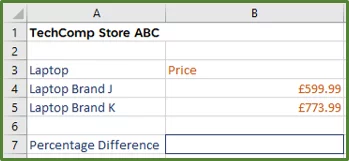
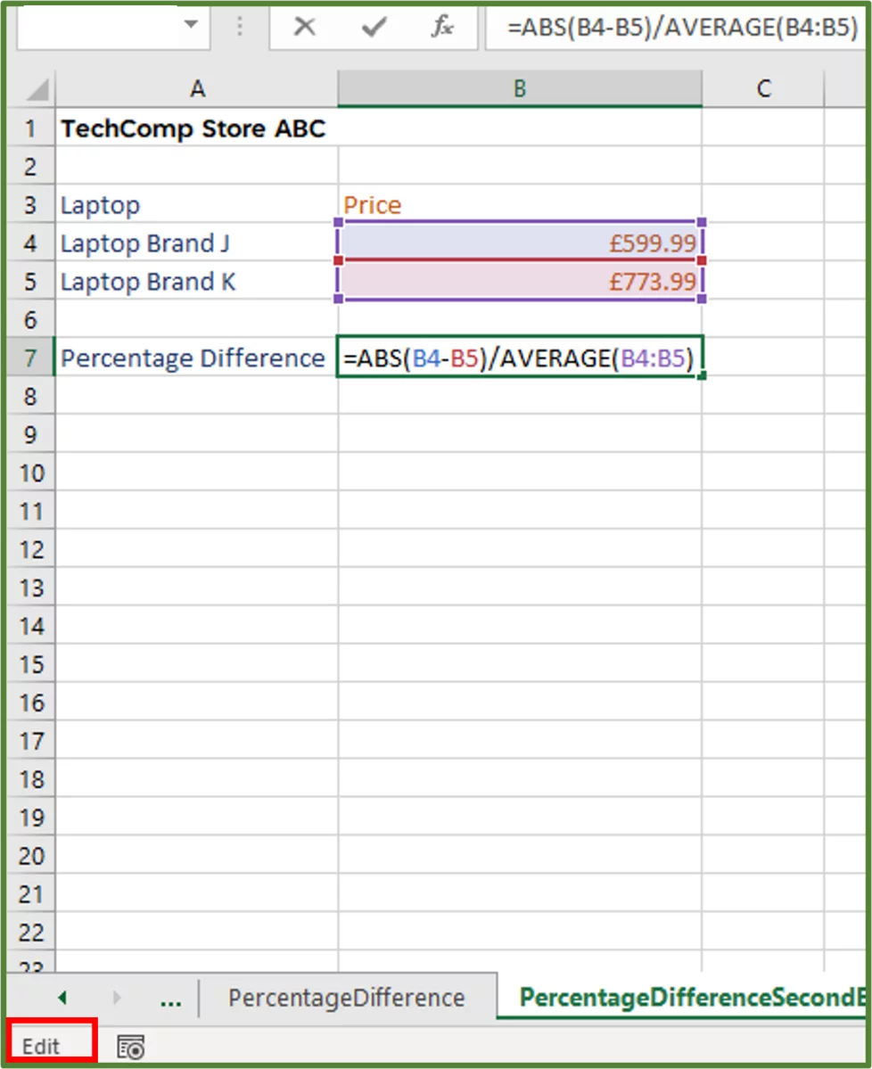
Let’s look at a slightly more complex example. We are still looking at laptop brands at the same store.

We want to calculate the percentage difference between Brand J and Brand K’s prices. The order in which we enter the two values into the formula doesn’t matter.

1)   So, we enter the following formula in cell B7.

=ABS(B4-B5)/AVERAGE(B4:B5)

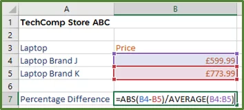
Note: Since we are interested in the difference between the two prices and one is not more important than the other, it doesn’t matter in which order we subtract.

For more Excel Data Tips, read our guide on Forecasts in Excel here.

Due to us subtracting the price in cell B5 from the price in cell B4, we get negative values. We can ignore the negative sign or use the ABS Function in Excel to return the absolute value of the number. In this case, we used the ABS Function as part of our formula.

2)  Press Enter to get the following.

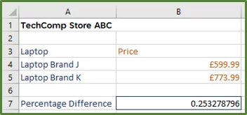
3)   With cell B7 selected, press CTRL+SHIFT+5 on your keyboard to apply percentage format.

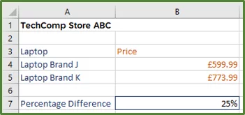
The percentage difference between the two values is 25%.

Now this value is expressed we can use it for whatever we like, such as formatting all cells with a high percentage difference. Read our guide here on Conditional Formatting here.

Calculating Percentage Change In Excel

You may have times when you want to compare an older value to a newer value. In these situations, you would use the percentage change calculation.

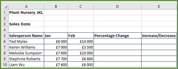
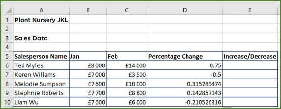
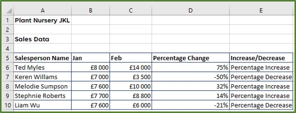
Let’s look at an example. We have a hypothetical plant nursery company and the sales data for each salesperson recorded for January and February.

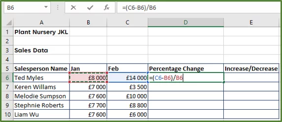
So, the percentage change for each salesperson would be calculated by using the following formula.

(Newer Value – Older Value)/Older Value. We would then apply the percentage format to the result.

1)   So, in cell D6, enter the following formula.

=(C6-B6)/B6

2)  Press Enter.

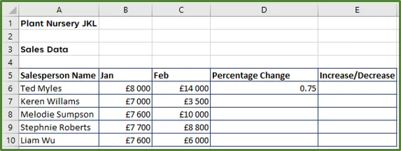
3)  Since we used relative cell references, we can drag the formula down the column.

This post covers Absolute Relative and Mixed Cell references.

4)  Now select cells D6:D10 and with the range selected, go to the Number Group on the Home Tab and choose Percent. Adjust the number of decimal places as needed.

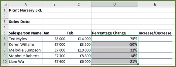
5)   Now, in this case, we are interested in showing the negative signs as well. For the first salesperson, we note that there has been a 75% percentage increase in sales. There has been a 21% percentage deccrease in sales for the last salesperson.

6)  So, we will use column E to highlight where there has been a percentage increase or decrease.

7)  So, with cell E6 selected, enter the following formula.

=IF(D6>0,”Percentage Increase”, “Percentage Decrease”)

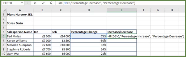
8)  Press Enter.

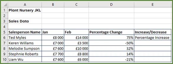
9)   Since we used relative cell references, we can drag the formula down the column to get the following.

Want to automate the process of calculating percentage differences? Read another great guide here on Creating A Macro In Excel.

Troubleshooting With Percentage Differences

If you encounter errors with your percentage difference formulas, it’s more than likely due to incorrect cell referencing.

So, one way you can check, is select the cell with the formula and press the F2 key to verify the references. This, will take you into Edit mode. You can press ESC to exit Edit mode.

We cover how to audit Excel formulas in this article. Read on for more help on this issue.

Learning Objectives

You now know how to:

• • Calculate Percentage Value in Excel
  • Apply Percentage Value Formatting
  • Calculate the Percentage Difference between two values in Excel
  • Calculate the Percentage Change between two values in Excel

Conclusion

The percentage difference is a helpful indicator when comparing values of the same type that are not more important than one another.

This, is a good formula for both beginner and advanced Excel users to know.

Special thank you to Taryn Nefdt for collaborating on this article!