
Excel For SEO – Basic Training Guide
Contents
Excel has every data analysis tool that you’ll ever need.
That’s great if you know about all of them.
You can focus on the fun stuff and get Excel to do the heavy lifting.
Our Microsoft Excel course has been delivered to many SEO’s over the years!
The questions and ‘ah ha!’ moments are the same each time.
If you are spending ages processing your data? This is your guide.
Let’s break down our 8 steps to getting in control of your data!
Step 1 – Working With Tables Of Data
Download data from any SEO tool, and it will come as a spreadsheet. To the layman, this is a table of data.
First things first. There is a difference between a table and a spreadsheet in Excel.
Unless you tell Excel that you have a table of data, it will assume that you just have a spreadsheet of data.
If you tell Excel that your data is a table, it will automatically format it and add certain functionality to it.
For this example, let’s use part of a download from Google Search Console.
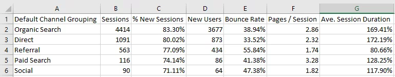
Excel does not automatically view this as a table.
To tell Excel that you want this data to be treated as one table:
The quick way is to highlight a section of it and to then click CTRL+T.
Alternatively, you can highlight all of your data and then go to the Styles group in your toolbar and click Format as Table button.
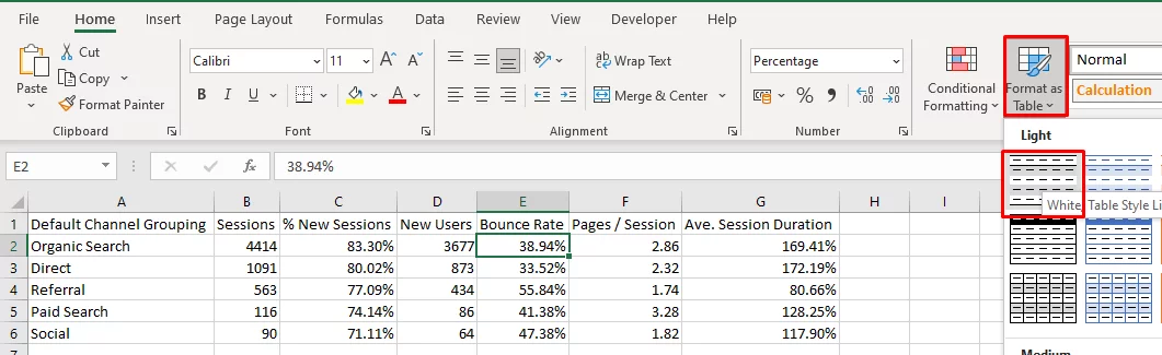
A drop-down box will then ask you how you would like to your data to be formatted.
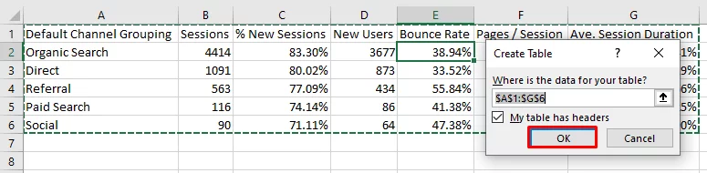
Once you have chosen the style of table you would like, a dialogue box “Format As Table” dialogue will appear.
This will ask you to confirm that it has selected the appropriate data.
It will also ask whether your data has headers included within the selected area.
The outline of your table of data will also be marked with a moving dashed line on the spreadsheet, making it very easy to check that Excel has selected the correct data.
When you click OK, you are left with the below. Mentioned above, the specific design is the one that you chose earlier in the process.
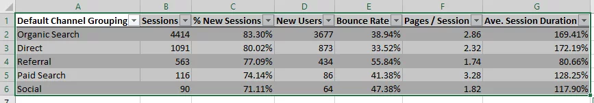
Your data is now a table. It will now be much easier to work with and manipulate.
As you can see above, Excel automatically adds filter buttons (highlighted above) to the titles of each of your columns. The uses for filter buttons are covered below.

You will notice that now every time you click on any cell within your table, a custom tab will become available. This is show above.
Many of these functions are beyond this article.
Now that Excel knows that you are working with a table of data, it’s time to see what we can do with it.
Step 2 – Formulas & Functions
1. DEDUPLICATE – Remove duplicates from your data
Deduplicate allows you to very quickly check for and remove duplicated data.
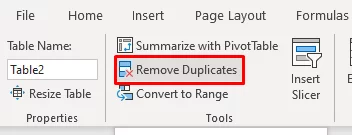
Using Table Tools makes this extremely simple.
Click anywhere within your table to activate the ‘Table Tools’ tab. Click ‘Remove Duplicates’.
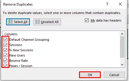
Excel now asks you which columns it should look for duplicates in. It will remove rows where the data in the ticked boxes is duplicated. Take care.
Assuming that you are concerned that you have identical rows of data, you need to tick each box as you are concerned about completely duplicated rows.
You can see in the screenshot below that I have duplicated three rows for the purposes of this example.
Unticking some of the boxes would allow you to remove rows which are duplicated only on the ticked rows.
Continuing on with our example, if we now click ‘OK’, Excel will automatically remove the three duplicated rows.
Excel will always retain the first row of the data and remove the subsequent duplicates.
It will also tell you how many duplicated rows that it has removed.
SEO Application:
This is generally used where you’ve got two or more datasets which aren’t complete and you want to combine them into one ‘master’ dataset.
For example, when preparing for a site migration creating a master URL list can involve combining data from Google, ScreamingFrog, Majestic etc etc.
2. SORTING DATA – Order Your Data By Date, Alphabetically or Numerically
Excel’s sort function allows you to reorder your data by the values in one or more of the columns.
The fastest way to do this is to use the filter buttons that appear at the top of your table.
Simply click on the button and a drop down box will appear.
The first two options will allow you to sort that column of data.
As can be seen below, if the data is numerical it will offer “Sort Smallest to Largest” and “Sort Largest to Smallest”.
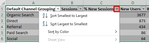
If it is text or date data then it will offer the relevant options so “Sort A to Z” or ‘Sort Oldest to Newest”.
It is possible to carry out multiple sorts, sorting first by one column and then by a second column. See further reading below for more details.
SEO Application:
Sort makes working with large spreadsheets of data far quicker. It has a huge number of uses.
For example, when looking at inbound metrics data from Majestic and Moz this is the quickest way to order your data by the highest linking domains, Moz rank etc.
Similarly if you’re looking at broken internal links via a 404 export from ScreamingFrog it is often easier to spot patterns and work through errors when the data is sorted by destination URL.
3. FILTER – Only Show Data That Meets Your Criteria, Hide The Rest
The FILTER Function is a natural follow on from sorting data. It lets you hide any data that doesn’t meet the criteria that you set.
This makes it much quicker and easier to work with your data, especially when you have a big dataset.
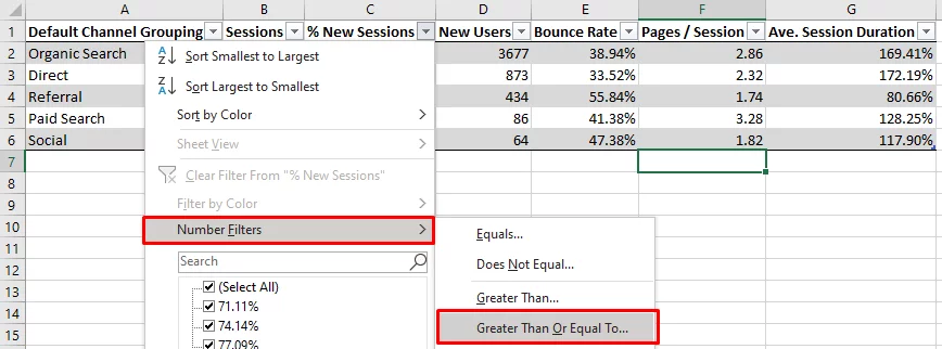
For this example we’ll use the filters to find only those traffic sources which have sent our site 100 or more New Users during the period.
Again you click the Filter icon at the top of your row but this time you look further down the menu that drops down.
First check that you don’t have any existing filters applied. You do this by checking that the “Clear Filter From “New Users”” option is not ticked.
This option will then only show in faded text as in the image below.
Next click ‘Number Filter” and a large menu will drop down. Choose ‘Greater Than Or Equal To’.
You can then insert your choice in the ‘Custom AutoFilter’ dialogue box. As you can see you could make your query a fair bit more complex if you choose.
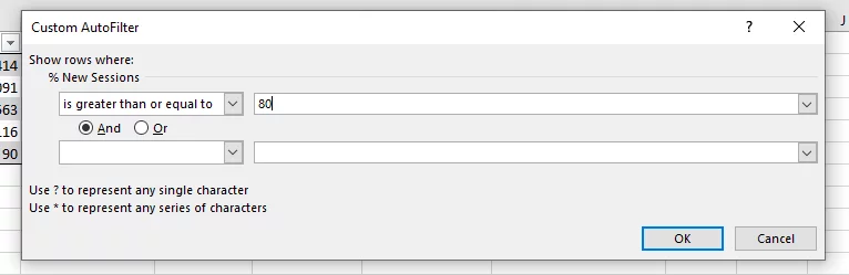
This would give the result.
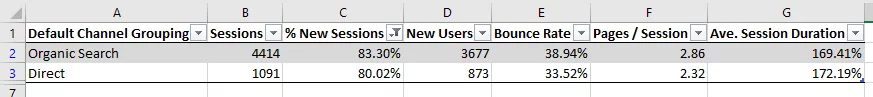
As you can see the filter icon at the top of Column D has now changed to show that that is the column which the data has been filtered by.
Also row numbers are now shown in blue, not the default black, and aren’t continuous as not all rows are being shown.
For more complex details, check out our guide to advanced filters in Excel here.
SEO Application:
Filter has a urge number of potential users, similar to Sort above.
Examples of SEO uses include sorting site errors by response code, finding duplicate metadata, looking at broken links by target URL.
It is also a useful way to search a specific column. For example, if you want to see all of the queries which relate to Excel in your Google Search Console download.
You would click the filter button in the header of the ‘Query’ row but then click into the search box and enter “Excel’. This looks for cells that contain Excel anywhere.
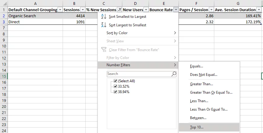
Finally another great one for looking at CTR is using the “Number Filter” and then using the ‘Above Average’ and / or ‘Top 10’ filters.
This will very quickly show you what your top performers are.
4. TOTAL ROW – Sum, Count Or Get The Average Of A Column Of Data
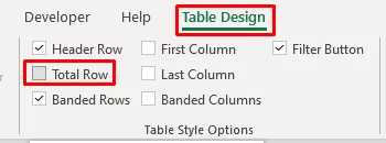
Total Row allows you to very quickly summarise the data in your table. In order to activate Total Row simply click anywhere in your table.
This will activate the ‘Table Tools’ tab. Next click ‘Total Row’. This will automatically add a ‘Total’ row at the bottom of your data.
It will also add a sum total to the new bottom right cell of your table.
Be careful of this statistic.
As you can see in the example below it’s not always the most useful, here it has summed the positions data!
Clicking in any of the other cells in the total row will trigger a dropdox box from which you can simply choose the statistic that you would like Excel to calculate.
SEO Application:
This offers a very quick way to summarise your data.
For example if you need to know the total number of impressions generated by queries containing ‘Excel’ from your Google Search Console download
You could even use your average CTR for queries containing ‘Excel’.
5. COUNTIF – Count How Many Times Something Appears In Your Data
Countif allows you to count how many times something appears in your dataset.
It will return a number which is the number of times that the string your are looking for has been found in your data.
=COUNTIF(range,criteria)
range – the group (usually a list) of cells that you want to search through
criteria – what you are searching the range for
SEO Application:
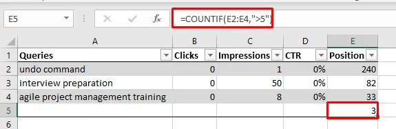
Countif is great for categorising data. An everyday SEO example would be calculating how many pages you have that rank at position 5 or higher.
Alternatively if you’d like to know how many pages get more than 10 or 50 or 500 visitors it will do that for you.
In conjunction with Len(see Chapter 2) it’s also an easy way to see how many pages have URLs longer than 70 characters.
Lets keep going with our Google Search Console query download and find out how many queries we rank at better than position 5 for.
6. SUMIF – Sum Only The Data That Meets Your Criteria
Sumif is very similar to Countif. This time it will find the sum of the contents of the cells that meet your defined criteria, rather than just counting them.
=SUMIF(range,criteria,sum_range)
range – the group (usually a list) of cells that you want to search through
criteria – what you are searching the range for
sum_range – does not need to be included. If it isn’t then SUMIF will sum the cells that meet your criteria. If it is, then SUMIF will sum the corresponding cells in this range, not in the range you defined earlier.
SEO Application:
Sumif is another very useful formula. It is doubly so when combined with Countif (see above).
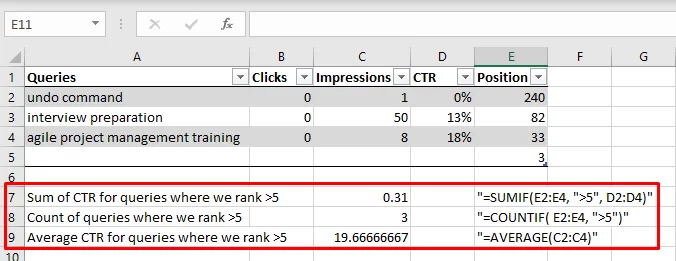
Continuing with our previous data we calculate our average CTR for queries where we rank 5 or better.
The screenshot below shows the calculations you would need.
Note that the highlighted section of the SUMIF formula is where it is summing items from a different column (column D) to the one that it is checking our ranking for (column E).
7. AND – Check if two conditions are both met by your data
AND is an extremely useful function, although mostly when used with other functions rather than on its own.
It allows you to find out if two (or more) conditions are met by your data. It will return TRUE if both (or all) of the conditions are met and FALSE if any of the conditions aren’t met.
=AND(logical test 1, logical test 2…..)
logical test 1 – the first test
logical test 2 – the second test. You can continue to add as many further tests as you like, so long as each one is separated by a comma.
SEO Application:
And can be used in an incredibly wide variety of ways. Finding data between two dates. Finding pages that only have a bounce rate between two values.
Finding pages that have a bounce rate above / below a certain threshold and duration above / below a certain amount. AND can do all of these and more.
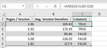
For example, which pages do visitors love most.
Continuing with our example data lets see which landing pages have pages per session of more than 2 and also an average session duration of less than 2 minutes (120 seconds).
8. OR – Check if either of two conditions are met by your data
Or is another extremely useful function. Similarly to And it is often used with other functions.
It allows you to find out if any of your two (or more) conditions are met by your data.
It will return TRUE if any (or all) of the conditions are met and FALSE if all of the conditions aren’t met.
=OR(logical test 1, logical test 2…..)
logical test 1 – the first test
logical test 2 – the second test. You can continue to add as many further tests as you like, so long as each one is separated by a comma.
SEO Application:
OR has a huge number of uses.
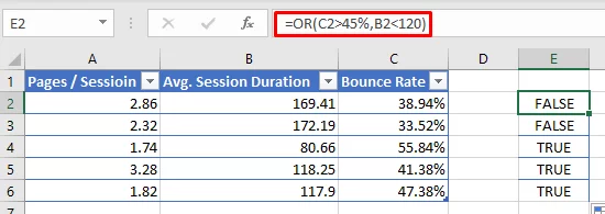
For example, to identify which pages don’t perform well with visitors you might want to find which pages either have more a bounce rate of more than 45% or an average duration of less than 2 minutes (120 seconds).
9. IF – Make Excel do one thing if one condition is met and another if it isn’t
Once you master If you’ll wonder how you lived without it.
It allows you to tell excel to do different things based on if one condition is met or not.
=IF(logical_test,value_if_true,value_if_false)
logical_test – the test that you want to apply to your data
value_if_true – the result of the formula if the test is met.
value_if_false – the result of the formula if the test is not met.
IF functions can also be put inside other IF functions, this is called a nested function. This allows you to apply more than one test to your data.
SEO Application:
IF functions can be incredibly useful. It’s so flexible there are potentially hundreds of examples of how it could be used.
It allows you to very simply categorise and manage data.
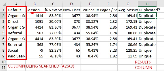
For example, if you want to see where data is duplicated but not remove it, it can do that very simply.
Using the data that we used for the deduplicate example above we can add a line to the spreadsheet to show if the data is duplicated.
The formula used below looks through cells A2 to A9.
If it finds the result in A2 more than once then it inserts the word Duplicate, if it finds the entry only once then it inserts Unique.
The $’s are added into the formula so that the range of cells searched doesn’t change when the formula is copied down.
This is an example of absolute cell referencing, which is a very helpful tool.
10. VLOOKUP – Find a specific row in your table and return a piece of data
VLOOKUP allows you to very quickly search for specific pieces of information in large tables.
It lets you specify the value that you would like Excel to find in a certain column.
You can then ask it to return a different piece of information from that row.
=VLOOKUP( lookup_value, table_array, col_index_num )
lookup_value – the value that you want to search for in the first column of your data
table_array – the table that you want the formula to work with
col_index_num – the number of the column in the table that you want the data from
There are a few caveats with VLOOKUP functions:
- It will only search in the first column of your data. Remember, you don’t have to specify your entire table of data if this is going to cause an issue.
- You need to sort the first column of data in your table.
- It requires an exact match. So if you search for “Excel” and your cell contains “Excel “ (note added space) the formula will not find a match.
- It will not find multiple matches. It will return the first match that it finds and ignore others.
SEO Application:
Given how many tables of data SEOs work with this has hundreds of uses. One of the main ones is combining tables.
If you insert the formula into a column in table A. It allows you to use a value from table A to find data for that value in table B.
A practical example would be that it allows you to quickly match adword volumes and Moz data when doing keyword research.
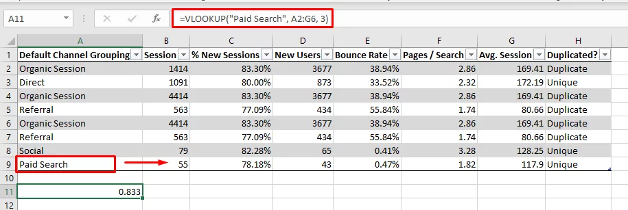
Using a simple example. We’ll just extract a value from a simple Google Analytics table that we used earlier in the article.
As the image shows, Excel searches down the first column of the table (A2:G6) until it finds an exact match for “Paid Search” and then looks across and extracts the value in column 3 (column C) of that row.
Step 3 – Working With Text And URL Strings
Excel works pretty well with text if you know how.
However, to the uninitiated working with text in Excel can be very painful and manual.
Many SEO tasks involve working with text and almost all SEO data relates to a URL.
This section focuses on how to manipulate and work with text and URL strings. The ability to manage these quickly will speed up your work hugely.
We will talk about strings a lot.
To avoid any confusion a string is just short for a ‘string of text’ and means any cell which contains some text of any sort, although it usually means words, rather than numbers.
Also a quick pro tip before we get started.
If you want to move to another line but while in the same cell you use ALT + ENTER. Pressing enter will move you to the next cell down in the same column
1. LEN – How Many Characters Are There In A String
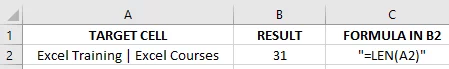
LEN calculates how many characters there are in a string or block of text. Note that it will include the spaces within the text if it is more than one word, or has a space before or after it.
| =LEN(text) |
text – the reference for the cell containing the string or block of text, or the text itself.
SEO Application:
Checking that your title tags aren’t more than 55 characters, your meta descriptions more than 155 characters and double checking the length of your URLs.
2. CONCATENATE – Join text strings together
CONCATENATE allows you to combine any number of text strings together to create one new text string. It does not add spaces between the items to be combined together.
| =CONCATENATE(text1,text2,text3….) |
text1 is the reference for the cell containing the first piece of text to bring into the combined string. It can also be a piece of manually entered text between speech marks.
text2 and onwards are optional
NB – if you would like to add spaces between your blocks of text, as below, get CONCATENTATE to add a space.
SEO Application:
This is one of the most widely used SEO formulas.
Google Analytics data exports don’t include a URL’s TLD as standard. Concatenate can quickly add the TLD if it is needed.
This is also useful for preparing HTACCESS redirect rules.
When preparing an htaccess file concatenate can save hours by grouping url, the redirect rule and destination in one statement.
Other uses include creating lists of keywords and potential search terms when you need to combine various terms.
Similarly, when you are reviewing your URLs this can be extremely useful.

3. TRIM – Remove excess spaces
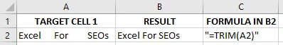
The TRIM Function will remove all excess spaces from a cell.
It will remove any spaces before and after the contents of a cell.
It will also ensure that there are only individual spaces between words in the cell.
| =TRIM(text) |
text1 is the cell containing the text to be trimmed.
SEO Application:
This will save your sanity if you’ve ever downloaded a large amount of data and found that spaces at the start of the cell contents mean that it won’t sort properly / adjust properly.
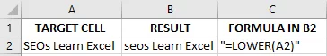
4. LOWER – Make all text lowercase
LOWER is very simple in that it converts all letters in a cell to lower case.
| =LOWER(text) |
text is the cell containing the text to be trimmed.
SEO Application:
This very quickly cleans up downloads of search terms that can be very strangely capitalised. Also if you want to ensure that you haven’t got any capitals in a list of URLs this is a great way to do that quickly.
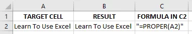
5. PROPER – Capitalise first letter of words
PROPER converts the first letter of each word in a cell into a capital letter.
| =PROPER(text) |
text is the cell containing the text to have initial capitals added to it.
SEO Application:
This is the quickest way to ensure that all of your page titles are capitalised if you’re working on a bulk download of a site in Excel.
Although not strictly SEO it’s also useful for Adwords copy.
6. LEFT & RIGHT – Extract a set amount of text from the left or right of a cell
LEFT and RIGHT will return a set number of characters starting at the left or right, respectively, of a cell.
| =LEFT(text,num_chars) OR =RIGHT(text,num_chars) |
text is the text to be worked with
num_chars is the number of characters to be extracted (from the left or right)
SEO Application:
LEFT is also useful when wanting to isolate just the domain names from a long list of sites. This is done in conjunction with SEARCH to find the first / after https:// – see example below.
RIGHT can be used to remove the domain leaving you with just a list of pages, as below.
It can also be used to find domains from email addresses by retaining only the section to the right of the @. Again this is done in conjunction with search.
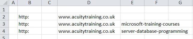
NB – 32 is the number of characters in “https://www.acuitytraining.co.uk/”
7. MID – Find and extract a defined part of a string
MID will find and extract a certain number of characters from the middle of a string.
| =MID(text,start_num,num_chars) |
text is the text to be worked with
start_num is the character at which the piece to be extracted starts
num_chars is the length of the text to be extracted in characters.
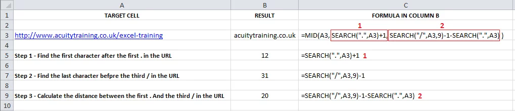
SEO Application:
MID is often used in conjunction with SEARCH, where SEARCH is used to define both start_num and num_char in a long list of URLs.#
Examples of where it is used include extracting just the domains or first level directories from a list of URLs, extracting duplicates with HTTPS and finding indexed/able URLs from a list generated by internal search.
8. SEARCH – Find A String Or Number
The SEARCH Function will find a letter or string within a larger piece of text. It returns a number that is where the first character of the string you are searching for appears.
In the event that it can’t find what you’ve asked it to it will return #VALUE, this doesn’t mean that there is an issue with your formula.
There are a couple of things to be aware of with SEARCH:
- It will find the FIRST instance of whatever you ask it to find.
- It is NOT case sensitive. If you need to find something specifically containing a capital letter or letters then use FIND.
- SEARCH allows you to use wildcards which represent any character. So ?EO, could be SEO, CEO or any other combination ending EO.
This means SEARCH doesn’t work with URLs containing “?”. Again in this event use FIND which doesn’t suffer this problem.
| =SEARCH(find_text,search_text,start_num) |
find_text is the text to be searched for
search_text is the text to be searched through
start_num is an optional input. It allows you to start the search not at character 1.
SEO Application:
SEARCH is often used in conjunction with other formula functions.
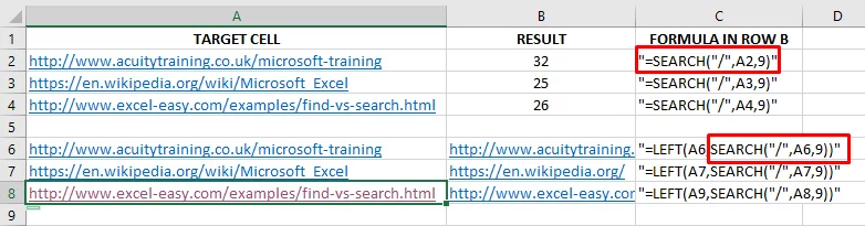
For example if you have a list of URLs where you want to retain only the domain name.
You would use SEARCH to find the third forward slash in the URL and then use LEFT (covered below) to retain only the number of characters that you had found with your search function.
The example below shows how to use SEARCH to find the third forward slash in the URL, by starting searching at character 9 (allowing for an SSL site).
Below that it shows how you can use a SEARCH function in a LEFT formula (see red boxes) to retain only that number of characters of your URL. Effectively just leaving the domain name.
Another useful trick with SEARCH is to use the fact that if it can’t find your string then it will return #VALUE. So if you want to exclude all entries that don’t contain something then you can use SEARCH and then exclude the lines that return #VALUE.
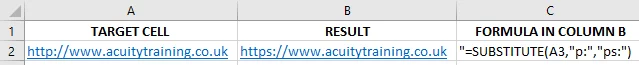
9. SUBSTITUTE – Swap one piece of text for another
SUBSTITUTE lets you find a piece of text and change if for another piece of text.
If you choose to replace a piece of text with a blank then this just serves to remove that text. SUBSTITUTE will change each instance of the text you ask it to find and replace, unless you set it to do otherwise, see instance below.
The “Find & Replace” functionality in Excel could be used to do this but SUBSTITUTE allows you to keep your source data intact.
| =SUBSTITUTE(text,old_text,new_text,instance) |
text – the existing text to be worked with
old_text – the piece of text to be searched
new_text – the piece of text to be inserted in place of old_text
instance is optional. It is the numbered instance that you would like to SUBSTITUTE. If you would like only the second instance of old_text to be changed you should use 2.
SEO Application:
SUBSTITUTE is great for changing one small part of a standard set up.
So setting up redirects when moving to HTTPS or moving domains, or replicating keywords, titles etc for different variations of a product Eg white shirt, green shirt, red shirt.
10. TEXT TO COLUMNS – Split the contents of a cell across a number of cells
TEXT TO COLUMNS lets you split the contents of a column of cells across a number of columns so that you can work on the sub-sections of that data.
It’s most easily understood by way of a worked example.
SEO Application:
TEXT TO COLUMNS is ideal for splitting out URL data into sub-categories.
This is particularly true if you want to sort the data by sub-category. For example if you want to look at metrics but at a sub-domain or folder level.
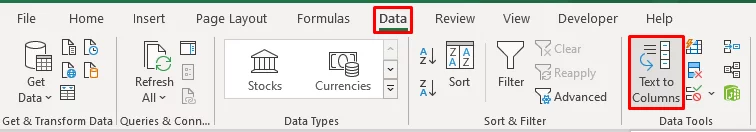
Start by highlighting the data that you want to split into columns.
Clicking the ‘Data’ tab and then the ‘Text to Columns’ button.
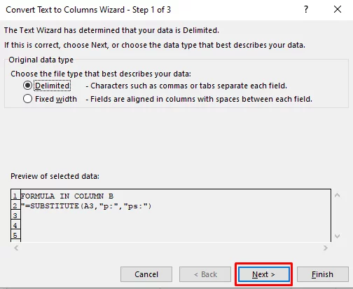
This will bring up the first of three dialogue boxes. It will show ‘Delimited’ checked. Don’t change this and click ‘Next’.
In the next screen you need to click ‘Other’ and then insert a / into the box next to it. This tells Excel that your data is split at each /.
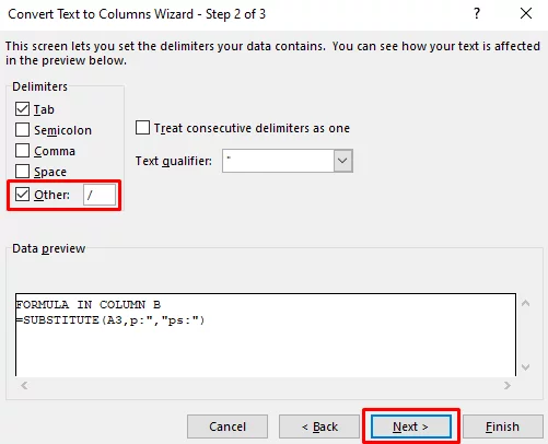
This will then take you to the final screen.
In general the ‘Format’ and ‘Destination’ will be fine and so you can just click ‘Finish’.
The only time it won’t be is if you are working with dates. In that case you will need to click ‘Date’ under format.
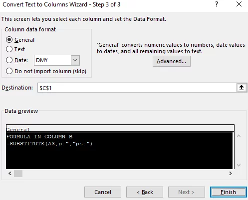
Once you’ve clicked ‘Finish’ your data will show as below and you’ll be able to get to work.
Step 4 – Working With Dates And Days
Working with dates in Excel is very quick and simple if you understand the basics well.
First of all, when working with dates you MUST make sure that the cells containing the dates are formatted to contain dates.
The number one problem for people working with dates is that they forget to check the formatting.
If you are working with dates and the cell contains a number DON’T panic. Excel stores dates as numbers, and then converts them to dates.
If you see a number it’s highly likely that you haven’t formatted the cell correctly.
Excel defines 1st January 1901 as day 1. This means that 1st November 2015 is 40,847. It is 40,847 days after 1st January 1901.
Excel contains lots of different date formats that you can choose from depending on what you would prefer.
To check the format of your cells, and ensure that you’re in a date format.
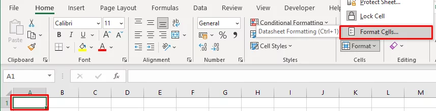
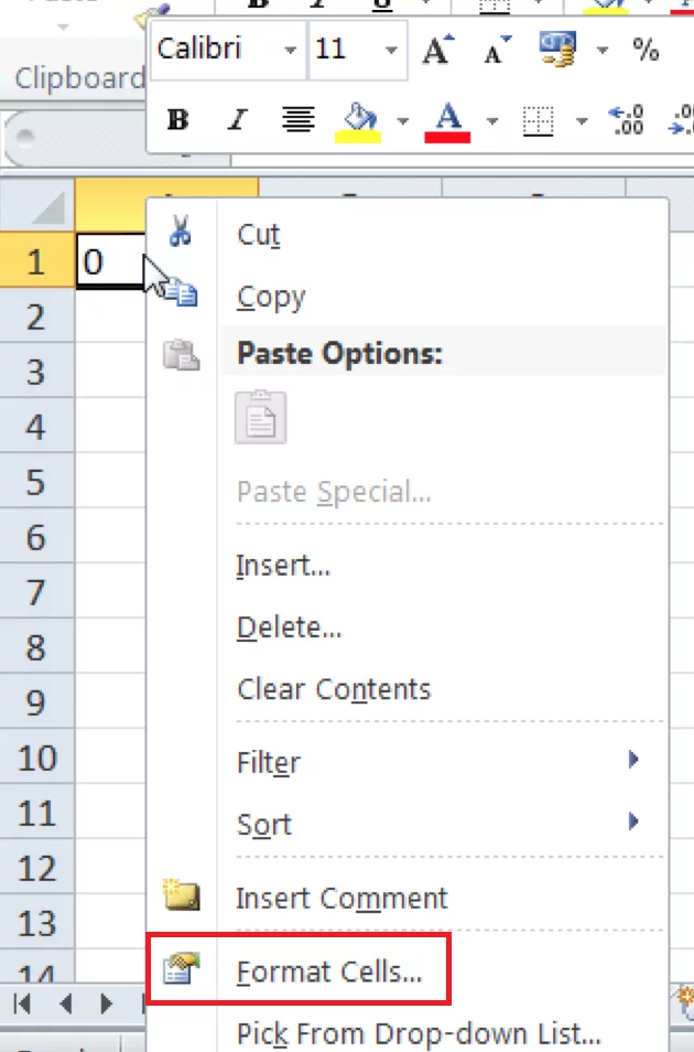
Firstly, select the cells you want to format. Next right click and select ‘Format Cells’ from the drop down menu.
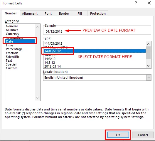
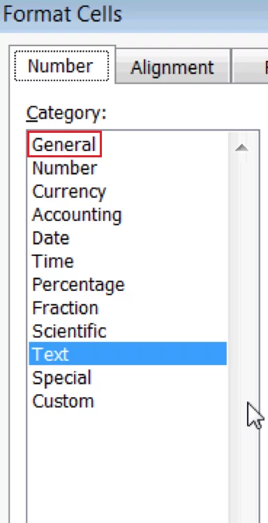
From the ‘Format Number’ dialogue box, select the ‘Number’ tab. Select ‘Date’ under category, on the left hand side.
Now choose the format that you would like for your dates from the right hand section.
If you’re unsure which format to choose, when you choose a format a preview of that date format will appear in the ‘Sample’ box above.
Having got your data properly formatted we can now start using it with Excel’s date formulas.
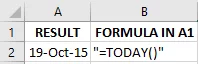
1. TODAY – Insert Today’s Date
TODAY simply inserts today’s date wherever it is.
| =TODAY() |
Note although the brackets are required for TODAY you do not insert anything between them.
SEO Application:
If you run the same reports daily then automatically inserting todays date can be a useful time saver.
If you set up your formulas correctly this will allow the calculations to automatically update themselves as the date changes. The image below shows how this works in practice.
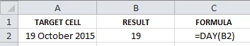
2. DAY – Convert A Date To A Day Of The Month
DAY allows you to convert dates to a numbered day of the month. This is very useful when calculating the number of days between two dates.
| =DAY(date) |
date is the reference of the cell containing the date that you want to obtain the day number for
SEO Application:
DAY allows you to easily calculate the number of days between two dates to work out average traffic numbers.
It is also often useful in formulas when carrying out more complex time calculations.
DAY is very simple to use as can be seen in the example below.
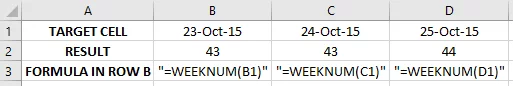
3. WEEKNUM – Find Out Which Week Of The Year A Date Is In
WEEKNUM allows you to find out what week of the year any date is in.
| =WEEKNUM(date) |
date is the reference of the cell containing the date that you want to convert to a week of the year
NB – By default all weeks run from Sunday to Saturday.
SEO Application:
This allows you to easily create weekly averages from daily data like a download from Google Search Console. This makes weekly comparisons simple to run.
For example if you wanted to know what weeks of the year 23rd – 25th of October 2015 fall in.
4. TEXT – Find Out What Day Of The Week A Date Is
TEXT allows you to convert a date into a day of the week.
| =TEXT(date,”DDD”) |
date is the cell reference for the cell containing the date you want to convert to a day of the week
“DDD” tells Excel how many letters of the day you would like shown.

SEO Application:
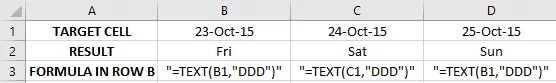
Allows you to easily correlate traffic variations with days in the week. By converting dates to days you can see weekly trends easily. You can also compare between weeks very easily.
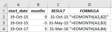
5. EOMONTH – Find Out Last Day Of A Month
EOMONTH finds the last day of the month for any given date. It will take the input date and calculate the date of the last day of that month.
It can also be used to take an input date and calculate the date of the last day of the month a set number of months before or after the given month.
| =EOMONTH(start_date,months) |
start_date is the initial date to be used for the calculation
months is the number of months forward (positive) or backwards (negative) that you would like the date calculated for. To calculate the end of the current month is 0.
NB – By default EOMONTH returns a number. This is a date but you will need to change the formatting of the cell to convert the number to a date.
SEO Application:
Extrapolating mid-month metrics (sessions, users, actions etc) to forecast full month metrics.
So for example, if the start date is 19 October 2015 and you want to find out the last day of the current month and the last day of the month in 5 months in the past and the future.
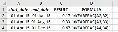
6. YEARFRAC – Calculate The Percentage Of A Year Between Two Dates
YEARFRAC lets you work out the percentage of a year that the period between two dates represents.
| =YEARFRAC(start_date,end_date) |
start_date is the earliest date of the two dates
end_date is the latest date of the two dates
SEO Application:
This is very useful when extrapolating year to date metrics (sessions, users, actions etc) to estimate full year metrics.
In this example we will use it to calculate what the amount of time between 1st April 2015 and 1st June 2015, and a couple of other pairs of dates in 2015.
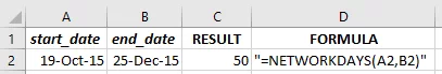
7. NETWORKDAYS – Calculate The Number Of Working Days Between Two Dates
NETWORKDAYS lets you work out the number of working days (Mon – Fri) between two dates.
| =NETWORKDAYS(start_date,end_date) |
start_date is the starting date of the period that you are interested in
end_date is the end date of the period that you are interested in
For people in countries that do not use Mon – Fri as the working week there is an additional NETWORKDAYS.INTL.
NB – NETWORKDAYS does NOT allow for public holidays.
SEO Application:
Used when extrapolating month and year to date metrics (sessions, users, actions etc) for businesses where working day traffic is very different to weekend traffic (Eg. most B2B businesses).
By way of example lets assume that you want to find out how many working days there are from 19th October 2015 to Christmas.
8. WORKDAY – Find Out What Date Is A Number of Working Days Away
WORKDAY calculates what the date is a certain number of working days (Mon – Fri) ahead or behind the entered date.
| =WORKDAY(start_date,days) |
state date is the start date for the calculation
days is the number of working days forward (positive number) or backwards (negative number) that you would like to calculate.
So if you would like to calculate what day is 23 working days backwards from 19th October 2015, or the date 18 working days forward.
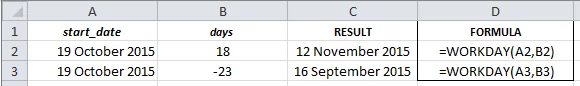
NB – WORKDAY does NOT allow for bank holidays and the like.
There is the option to manually input bank holidays that you would like to ignore (See this link for more details) but we find it is quicker to do this manually as it requires you to enter the dates you want to exclude numerically rather than as dates.
SEO Applications:
Workday is used for forecasting when certain metrics (number of actions) are likely to be hit for businesses where weekday and weekend traffic is very different. For example in a B2B business traffic is likely to be far higher during the week.
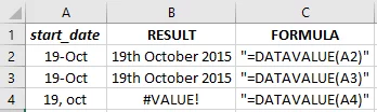
9. DATEVALUE – Convert Text Dates Into An Excel Readable Dates
Sometimes when you import your data into Excel the dates are just text strings. Converting the cell format to date will often prompt Excel to realise that the cell contains date data. However, if Excel doesn’t you face the boring task of manually amending the dates.
If this happens Excel has a pretty smart function DATEVALUE that may well fix the problem.
| =DATEVALUE(date_text) |
date_text is the reference of the cell containing the text based date information
This will often allow Excel to understand the text string. Obviously you need to look at it’s output very carefully to be sure that it has interpreted the string correctly.
NB – The output of DATEVALUE() is numeric by default. You will need to format the output cells (as above) to get a useful date output.
SEO Application:
This is a big time saver on the rare occasions that it’s needed which is why it’s been included.
It does occasionally happen that you are sent data that isn’t in an Excel readable formula / gets corrupted in conversion (from LibreOffice or Google Sheets).
To show the sorts of text that this will work on, see the examples below.
Step 5 – Errors and How To Fix Them
The joy of Excel is its sheer flexibility.
However, this flexibility means that you have to be sure to give Excel the data that it is expecting in the way that it is expecting it.
It can’t figure out what you are asking it to do, it just blindly follows the instructions that you give it – for better or for worse!
This section will show you how to understand and deal with the various error messages that Excel can produce when you have an issue.
Also, it will show you deal with some of the other frequent issues that can occur, like results appearing in unexpected formats (as dates not numbers, for example) or formulas not calculating.
There are 7 different types of errors that you will frequently get when using Excel.
Below we list each of the 7 and look at what causes them and so how you can fix them.
1. Circular Reference Warning Dialogue Box
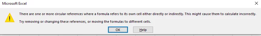
A circular reference dialogue box will appear if you have a formula that needs to use itself to calculate a result. This obviously doesn’t work. Luckily Excel picks up this error and warns you rather than going in an endless loop and crashing.
When you click OK Excel will automatically tell you where the circular references are. If you look at the bottom lefthand corner of your sheet it will show the cell that has a circular reference.
![]()
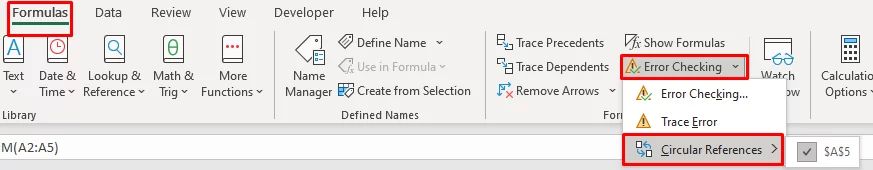
Alternatively clicking on Formulas, Error Checking and hovering over Circular references will show the cell / cells with circular references.
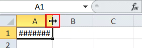
2. ##### Error
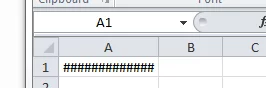
This is the simplest error that you will see, and it’s easy to fix.
Simply, this means that the number that the cell would like to display is wider than its column.
The fix is clearly either widening the column or reducing the space required by the number.
Columns can be widened in two ways.
This can be done manually by clicking and dragging the right border of the column header to make the column wider.
To speed this process up you can double click on the right border of the column header.
Excel will automatically resize that column so that it will fit the widest cell in that column.
This can be very useful when dealing with large amounts of data.
3. #DIV/0! ERROR
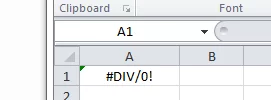
This is another relatively simple error to fix.
This is telling you that your formula is trying to divide something by zero, which doesn’t work mathematically, as it gives a result of infinity.
There are two fixes for this.
If your formula should not be dividing by zero, then you need to trace the cells that it is using. Once you have found the one which is showing zero, you then have the source of the problem. See tracing cell precedents below for more details on this.
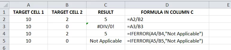
If everything is correct, it’s just that sometimes the formula will try to divide by zero, then you need to adjust the presentation so that people don’t think that there is an issue.
The screenshot below shows how using a simple IF formula, will allow you to show the result of the calculation, unless it is trying to divide by zero. In that case, the cell will show “Not Applicable”.
4. #VALUE! ERROR
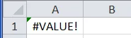
This error is generated when a formula is receiving data that is of the wrong type. For example, if you are trying to add a number and a date, or a date and some text. Excel has no idea what to do with this and so will give a #VALUE! error.
Again if you receive this error then you will need to trace that cells that the formula is using. Once you have found the cell which is containing the wrong type of data you will have identified the source of your problem.
5. #REF! ERROR
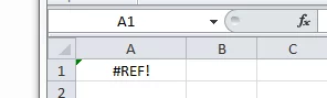
This error is generated when a formula is trying to access an invalid cell reference.
Generally this error is generated in two ways.
Firstly referencing a cell that has been deleted, and so Excel can’t find it.
For example, a formula references to another sheet in your spreadsheet. You then delete the worksheet, forgetting that that formula contains a reference to that worksheet.
Excel now doesn’t know what to use for that part of the formula and gives you an error.
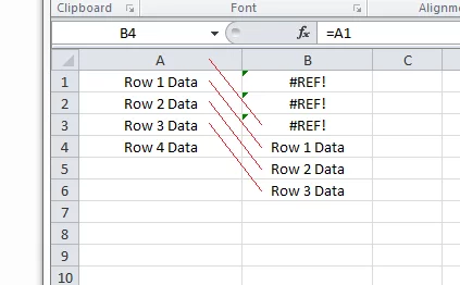
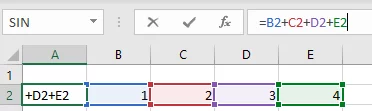
Secondly, referencing a cell that is off the spreadsheet. The example below shows a formula in row 5, that references a cell 3 rows above it.
If that is now copied up into rows 4, 3 and 2, when it reaches rows 3 and 2 it will be looking for cells that don’t exist.
Again, Excel won’t know what to use for that part of the formula and give you an error.
6. #N/A ERROR
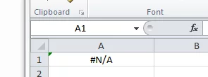
This error shows that a required value is not available to a function or formula. This generally occurs when using a LOOKUP or MATCH function. If the formula is looking for a specific number or piece of text in a list and that number or text is not in the list then it will show a #N/A error.
7. #NAME? ERROR
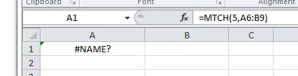
When Excel finds text in a formula (after an = sign) it will try to interpret is as a formula name, a named range of cells or a cell reference. If it can’t recognise the text as one of these three possibilities it won’t know what to do.
This error is generally generated in one of two ways.
Firstly, a simple typo.
For example, if you want to use a MTCH function and accidentally type MTCJ then Excel will not recognise this and will give you this error to explain that it doesn’t understand the formula.
Secondly, some formulas require that you put text between double quotes. If you forget to do so then it will give you this error.
Fixing Errors
If your Excel formula is giving you an error then start by understanding what the error message is telling you. This will give you some very good pointers about where to start looking for the error.
If you look at your formula and can’t see, using the clue that the error message gave you, where the issue lies then you will need to go through each element of your formula.
So double check for each part of the formula that it is spelt correctly, the reference is valid, if it is text should it be in double quotes etc.
There is really no short cut for this once you have exhausted the clues that the error message gave you.
This is generally very quick and straightforward with simple formulas. With larger formulas this can get quite tricky and time consuming. Luckily Excel contains a number of aids when you are error hunting which can speed things up markedly.
Coloured References
Firstly once you have inserted your formula into a cell, if you then double click on that cell it will show you the formula with each cell reference in a different colour.
The cell referenced will also then be bordered in the same color. This makes following cell references much quicker and simpler.
In the example below cell A2 has been double clicked.
Trace Precedents
In small spreadsheets with simple formulas, using the above works extremely well.
For large spreadsheets, you often can’t get the formula and the cells that it is referencing on the screen at the same time. When this happens, it can be confusing to remember what each cell is referencing.
If this is the case then using trace precedents is an easy way to see which cells a formula is referencing. It adds lines from the formula cell to its precedent cells, making following the formula far simpler.
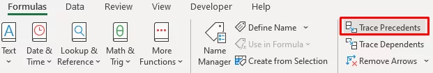
To find trace precedents, you click FORMULAS and Then TRACE PRECEDENTS, which is in the formula auditing tab.
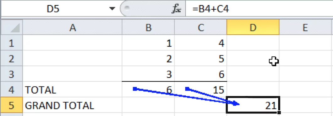
The first time that you click trace precedents, it will show lines to the direct precedents.
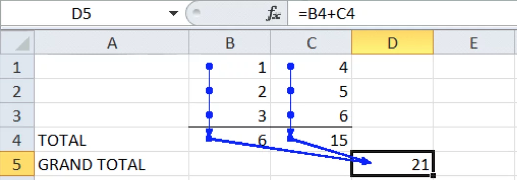
If you click trace precedents again it will show the precedents of the precedent cells that it has just highlighted.
First click of trace precedents button.
Second click of trace precedents button.
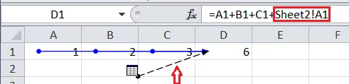
Trace precedents also works for cells in different tabs of a spreadsheet.
These precedents are shown with a black dotted line that points to a spreadsheet icon.
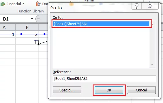
Double clicking on the dotted line will bring up a ‘Go To’ dialogue box.
The Go To dialogue box will list the offsheet cells that the formula references (in this simple case only one).
Click on the cell reference that you would like to see and then click OK and Excel will take you to the offsheet reference for your underlying formula.
Step 6 – Other Issues You Might Encounter
The Formula Doesn’t Calculate
Occasionally Excel will just show your formula in a cell, rather than the output of it’s calculation.
There are a few reasons why this might happen.
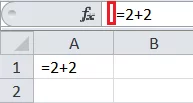
Firstly check that you don’t have a space or a single quote mark before the = sign. Both of these will cause Excel to show the formula. They are both easily done accidentally and tough to spot.
Here’s an example with a space in front.
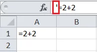
And here is one with an apostrophe in front.
Secondly, check the formatting of your cell. It might be that the cell is set up to show text and so is assuming that this is the text that you want it to display rather than the result of a calculation.
To fix this simply adjust the format of our cell to a number format.
Firstly, Right Click and choose Number Format
Then choose either General or Number from the dropdown menu.
If all of the formulas on the sheet are showing then check that you haven’t turned on the ‘Show Formulas’ option.
This can be done either by pressing CTRL+’ or clicking the ‘Show Formulas’ button which is in the formulas auditing section of your QAT.
Results Appear As Dates
Sometimes your formula runs without showing an error message but the output of the formula is wrong. For example, you are expecting a number and the cell shows a date.
If this happens it is because the format set for your cell is wrong. This often occurs because the column or row has been inserted.
When new rows and columns are inserted, they automatically inherit the formatting of the adjacent cells.
The simplest way to fix this is to change the formatting of your cell. Right click on the cell / cells with the incorrect formatting.
Right click and select Format Cells. From the tabs at the top of the ‘Format Cells’ dialogue box select ‘Number’ and then select ‘General’ under Category.
Step 7 – 17 Excel Shortcuts You’ll Use Daily
There are over 200 shortcuts in Excel. Most of them aren’t terribly useful.
The shortcuts listed below are the 17 most useful shortcuts.
| SHORTCUT | ACTION |
| CTRL + ↓ | This jumps you to the bottom of the current column of data that you are working on, provided that it doesn’t contain any blanks. This is very useful when working with very large spreadsheets. This also works for the other arrow keys if you want to jumpt to the far right, left or top of the current data that you are working with. |
| SHIFT + CTRL + ↓ | Pressing shift at the same time as CTRL and one of the arrows will allow you to select every cell from where you are currently to the end of your data. |
| CTRL + * | This selects all of your current data. The selection will stops where there is a completely blank row / column. |
| CTRL + : | This inserts the current time and date, which will not then change. This is a very quick way to time stamp a spreadsheet or other piece of work. |
|
F4 |
Pressing F4 repeats that last command that Excel carried out. If you need to do something repeatedly it saves a lot of clicking. For example, if you want to amend the format for a series of rows, right clicking on each one and then choosing the appropriate formatting each time can be a pain. This way you do it once and then highlight each row and press F4 which is far quicker. Once you’ve used this you’ll be addicted it’s a HUGE time saver. Be aware that this doesn’t work for absolutely every command but apparently it works for more than 90% of commands. So double check the first one. |
| F4 | When entering a formula if you want to add an absolute cell reference then press F4 while in part of the reference. This will change A1 to $A$1. Press F4 again and it’ll change to A$1, press F4 again and you’ll get $A1. |
| CTRL + Z | Just done something that isn’t right and want to quickly undo it? CTRL + Z will undo the last change that you made. Press it again and it’ll undo the change before that. Usually Excel will save your last 16 actions. |
| CTRL + R | If you’ve undone something or a series of things and wish you hadn’t then CTRL + R ‘Redo’ will take you back forward through the sequence. |
| CTRL + F | If you want to search through your data for a specific word, string or number then CTRL + F brings up a search box. Insert what you’re looking for and click ‘Find Next’. Excel will find the next instance of what you’re looking for. It will be in the highlighted cell. Click ‘Find Next’ again and it’ll find the next instance and so on. |
| CTRL + X | This cuts the contents of the current cell, or highlighted text, and adds them to the clipboard. |
| CTRL + C | This copies the contents of the current cell, or highlighted text, and adds them to the clipboard. |
| CTRL + V | This pastes the contents of the clipboard into the current cell. |
| CTRL + S | This saves your workbook. |
| CTRL + HOME | This will take you straight to cell A1 from wherever you are in your spreadsheet. |
| CTRL + END | This will take you to the last cell in your spreadsheet, so the righthand cell of the bottom row |
| CTRL + T | Convert range of data which contains active cell into a table. |
| CTRL + A | Select all of the current data in your spreadsheet. Press it again and it will select the sheet in which you are working. |


- Facebook: https://www.facebook.com/profile.php?id=100066814899655
- X (Twitter): https://twitter.com/AcuityTraining
- LinkedIn: https://www.linkedin.com/company/acuity-training/