The PMT Function – Master Excels Financial Tools!

Only a basic sense of the financial functions of Excel will help you get through most of your daily-life financial calculations.

Excel offers multiple financial functions including PMT, IPMT, and PPMT, all of which are designed to cater to the financial calculus needs of regular Excel users.

Did you know 98% of people have seen an Excel error cost their employers’ money? Mastering Financial Tools will help you minimize these mistakes! For more stats refer to our Excel statistics.

The article below should help you learn everything you need to know about the PMT function. So lets get to it!

Excel PMT Function

In all simplicity, the Excel PMT function belongs to the library of Excel financial functions. The abbreviation ‘PMT’ stands for the word ‘payment’.

Like in nature to its name, the PMT function is primarily designed to calculate the payments due against a loan. With that being said, you only need to populate your basic loan constants and variables in the PMT function and leave the rest to Excel.

 

Syntax

Syntax of the PMT function consists of five arguments.

 

Arguments

The five arguments offered by the PMT function syntax are broken down below.

• • Rate – This is the rate of interest applicable to the loan per period. It can take the form of a decimal number (0.1) or a percentage (10%).
  • Nper – This represents the number of payments to be paid over the period of the loan. In other words, the number of installments to be paid.
  • PV – PV stands for the present value (today’s value) of the loan. Simply put, it is the amount of loan you have received.
  • FV – [Optional argument] In contrast to PV, FV is the future value that represents the value of your loan on maturity. If omitted, Excel, by default, sets it to 0.
  • Type – [Optional argument] This argument specifies the type of payments i.e. advance or accrued payments. This argument can take two forms.

• • • Omitted or 0 – Accrued payments that fall due at the end of each payment period.
    • 1 – Advanced payments that fall due at the beginning of each payment period.

 

Return Value

The PMT function returns the payment for each period to be made against the loan.

It is to be noted that the return value against the PMT function in Excel would take a red color and the ‘Accounting’ format by default.

 

 

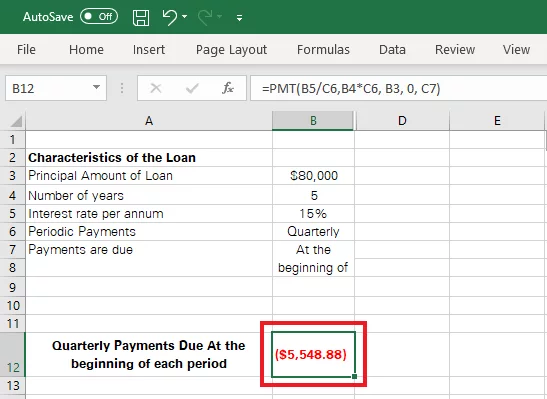
Also, you would find it to be enclosed in parenthesis as Excel gives back a negative value. This is because payments against the loan are to be debited to your bank account making it a cash outflow.

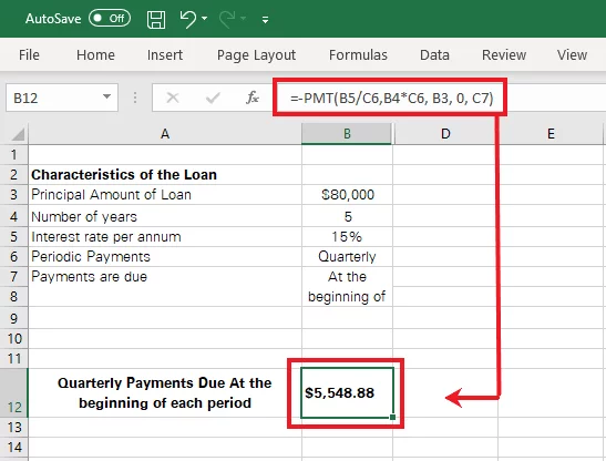
However, if you want the return value encased as a positive value, simply hop on to the formula bar and add a minus (-) sign before the value. Taking you back to a lesson from Grade 2 mathematics, ‘minus and minus make a plus’. Adding a minus sign before the value in the formula bar would turn it positive.

 

 

Functions Library

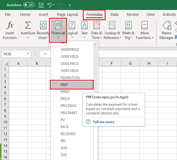
To quickly access the PMT function from Excel’s functions library, take the following route.

 

 

Why would anyone want to use the PMT Function?

Look into any office in the banking or insurance industry and you’ll see just how much the PMT function is used.

Mastering functions is a great way to get your foot in the door with financial jobs!

Even otherwise, the PMT function is of great help for students from the fields of business and finance. It rids users of the need to use pricey financial calculators or to memorize and apply the complex formulas for annuity and IRR.

Also, people from different fields of life can apply it to their daily life to better plan their financial borrowings and lending matters.

In addition to the PMT function, many other array functions of Excel can help you with most of your data sophistication tasks. Check out the FILTER and RANDARRAY function here.

 

PMT Function Use Cases

Listed below are a few common instances where the PMT function is massively used.

• Professors from a finance class might assist students in performing calculations for finding loan/lease payments for academic questions using the PMT function.
• As a banker, you may want to prepare reports for a specific loan product offered by your bank. PMT function combined with the drag and drop function of Excel can help compute the payment statistics for thousands of consumer loans in one go.
• Contractors and businessmen may use the PMT function to perform feasibility studies for the new projects they undertake. A smartly worked PMT function can help compute the break-even point for a given contract.

The PMT function is an easy way to work out finances for people who are not from the field of business and finance. For details on logical functions in Excel, go here!

 

Use PMT to calculate payments in Excel

Using the PMT function to calculate payments in Excel is fun. Let’s take a look into the example below to see how it works.

 

 

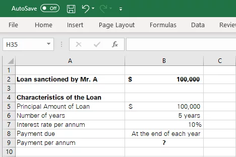
The image above contains the details of the loan taken by Mr. A. These details include the amount of loan taken, the interest rate, and the time when the installments fall due for payment. However, the amount of periodic payment is to be found.

Here’s how we can use the PMT function to find this.

 

Step 1:

To find the periodic payments to be made against this loan, the PMT function needs to be set up as follows.

 

• • The first argument for rate is set to the interest rate applicable to the loan i.e. 10%.
  • The second argument represents the number of annual payments to be made over the period of the loan. As the number of years for this loan is 5 and periodic payments are scheduled for every year-end, the total number of payments is 5.
  • The third argument for the present value of the loan is kept to $100,000.
  • The fourth argument for future value is omitted and will be automatically set to 0.
  • The fifth argument for the type of payment is omitted and will be set to 0 by default. 0 is used for accrued payments that fall due at the end of each period and the payments in the subject loan fall due every year-end.

 

Step 2:

Activate a cell, populate the above formula, and hit enter to see results as follows.

 

 

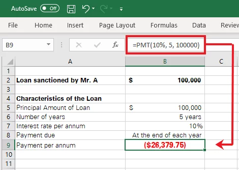
Excel has computed the periodic payment to be ($26,379.75). In short, an amount of $26,379.75 will be paid every year for up to 5 years before the loan is fully repaid.

 

Using PMT for Semi-annual, Quarterly, and Monthly payments

The above example contained a simple data set where the interest rate compounded annually, and the payments were also to be made annually.

However, it is often the case that interest compounds annually, whereas the payments are scheduled semi-annually, quarterly or monthly.

Before we talk about the additional changes to be made to the basic PMT formula for differently scheduled payments, it is essential to understand why is it even needed?

 

The concept of compounding!

Interest works on the science of compounding. In simplest terms, let’s say you take a loan of $100 at an annual interest rate of 10% and use it for one year. After one year, your payable is not $100 but $110 i.e. (Principal loan amount of $100 + Interest of $10 compounded over a year).

At the end of year 1, if you pay off $20, your payable now stands at $90 ($110 less $20). The interest would now compound to $80. This is what happens when payments are scheduled in line with the interest rate compounding period.

However, had you made the payment of $20 in the mid of year 1 and not at the end of year 1 when the interest rate compounded annually, your payable at mid of year 1 would have been $85 (Loan of $100 + $5 interest for half a year – $20 payment made).

In this case, would the interest compound at $85 since the mid of year 1? No, it would still compound on $100 until the end of a year. This creates a mismatch between the compounding period and the rate of interest.

To find the correct amount of payment in such cases, the following steps must be followed.

 

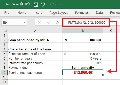
Semi-annual payments:

Semi-annual payments mean two payments a year. A simple way to work out the PMT formula is to make a two-step change to the formula:

• • Divide the first argument i.e. rate by the number of payments to be made in the year.
  • Multiply the second argument i.e. Nper with the number of payments to be made in the year.

As the number of payments in this instant case is 2, the PMT formula for the above example will therefore change as follows:

 

Press ‘Enter’ to see the results as follows:

 

 

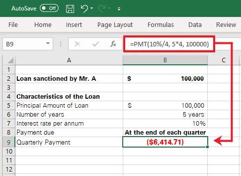
Quarterly Payments:

Quarterly payments mean four (4) payments a year (at the end of each quarter). Using the simple two-step change mechanism above, the PMT formula for the above example will change as follows:

 

Press ‘Enter’ to see the results as follows:

 

 

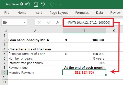
Monthly Payments:

Monthly payments extend to payment at the end of each month, making a total of twelve (12) payments a year. The PMT formula should be worked out as follows:

 

Press ‘Enter’ to see the results as follows:

 

 

Must Note!

It is to be noted that the foregoing adjustments to the PMT formula are only required to be made when there is a mismatch between the interest rate compounding period and the payment interval. No adjustment is required to be made if both of them are the same, for instance:

2 semi-annual payments of $100 are to be made when the interest rate is 12% compounded semi-annually.

 

How to make a PMT calculator in Excel

Before you sign up for a loan, it makes sense to search for and evaluate other available options.

A PMT calculator in Excel is a fun tool that will help you calculate the payments due for a wide variety of loans with only a click or two. The following steps will help you create your own Excel loan payment calculator.

 

Step 1:

Organize all the loan details in different cells, as shown below.

 

 

Step 2:

For the two variables that keep changing for different loans i.e. payment intervals and time when payment falls due, you may set up a drop-down menu as shown below.

 

 

To set up a drop-down menu, go to the Data Tab > Data Tools > Data Validation > Set up a list of options.

Step 3:

Once the data is set up, we need to set up a function that will automatically select the desired numeric value against each option. For instance, to compute monthly loan payments at the end of the period, we need to multiply the ‘Nper’ argument with 12 and set 0 as the Type argument.

To do this, you need to:

1. 1. Set up a key for the numeric values; and
   2. Work out the VLOOKUP Formula.

Setting up a key is relatively easier. All you need to do is, define each option from the dropdown menu and add a numeric value to it that will be used in the PMT function formula. Take a look below.

 

 

Step 4:

Next, you need to put in place a VLOOKUP formula that chooses the numeric value against each option. For instance, if we choose ‘Monthly’ against the Periodic Payments option from the drop-down menu, the VLOOKUP formula would automatically choose 12 against it.

To do so, activate any cell and compose the VLOOKUP formula as follows:

 

 

Under this formula, Excel would look up the value in B9 (any periodic payment type) against the values populated in the key for ‘Payments are due (Type)’. Based upon this, it will return the corresponding value from column 2 to the table array E9:F10.

See here how this works.

 

 

In the above image, the VLOOKUP function has returned the Column 2 value corresponding to the value “At the end of each period” which is 0.

Set up a similar formula for ‘Periodic Payments’ as follows:

 

 

Here is how this works.

 

 

Step 5:

Compose the PMT function as follows:

 

 

• • The first argument for rate is set to B5/C6. B5 contains the interest rate, whereas, C6 contains the number of periodic payments to be made each year.
  • The second argument B4*C6 represents the number of payments to be made over the period of the loan. It is the product of the number of years for this loan and the number of periodic payments each year.
  • The third argument is set to B3 which contains the present value of the loan.
  • The fourth argument for future value is set to 0.
  • The fifth argument for the type of payment is set to C7. The VLOOKUP formula working at the back of C7 will automatically update it to 0 or 1 depending upon the variable chosen from the drop-down menu.

 

Pro Tip!

This is important to note that the spelling and words used in the source data and the key must be the same for the VLOOKUP function to work.

 

Step 6:

For better labeling you may want to set up an auto-update formula in the label that presides the amount of payment as follows:

 

 

This involves the use of the concatenate function. Now, like the options from the drop-down menu update, the label updates automatically.

 

Step 7:

Your PMT calculator is all set to rock. All you need to do is, add the relevant data for different loans and set the variables from the drop-down menu accordingly to get instant results as follows.

 

 

How does this work?

With the PMT calculator, you now only need to update the source data for different loan products, and Excel would calculate the future payments for you automatically.

For instance, to find the amount of payment due for a loan of $80,000 for 5 years at the interest rate of 15%, where the payments are due quarterly at the beginning of each period.

Set up all the variables in the Excel sheet, and you’re good to go!

 

 

Learn more about linking data in Excel here.

 

PMT Troubleshooting

If you think your PMT function is not working as intended or is giving back inappropriate results, you may want to check for the following common issues:

 

#VALUE! Error

The PMT function results in a #VALUE! error when one or more of the arguments to the PMT function are text values. As seen above, none of the arguments to the PMT function are in text form but numbers or percentages.

 

#NUM! Error

If Excel gives back #NUM! Error to the PMT function, check for the following two reasons:

• • Is the rate argument negative?
  • Have you set the number of periodic payments to zero?

 

Inappropriate results

At times, you might find the results of your PMT function to be inappropriate. Take a closer look at the formula to check if you’ve made a mistake dividing or multiplying the rate or the period.

 

Conclusion

That is how you can use the PMT function to calculate payments for different loan plans in Excel. Practice this function using different sets of data with payments falling due around different times of the year. Once you’ve mastered the PMT function, you’ll never want to revert to the old, complex methods of calculating loan payments through lengthy formulas.