Power BI Filter Context – How Measures Really Evaluate

Filter context is one of the most important and most misunderstood concepts in Power BI.

It is also the reason a single measure can return different values depending on where it appears in a report.

This article is written for users who already build measures, but still encounter numbers that change unexpectedly across visuals.

The goal is not theory for its own sake. The goal is predictability.

Once filter context is understood, measure behaviour stops feeling mysterious and starts becoming intentional.

What Filter Context Actually Means

Filter context is the complete set of filters applied at the moment a measure is evaluated.

Every visual in Power BI asks a question of the model. That question is never asked in isolation. It is always asked within a specific context that determines which rows are visible to the calculation.

Filter context can be shaped by:

• Fields placed on visual rows, columns, axes, or legends
• Slicers
• Visual-level, page-level, and report-level filters
• Cross-highlighting and visual interactions
• Row Level Security, which acts as a permanent background filter

Every DAX expression is evaluated within a context that defines which data it operates on. Filter context is one half of that evaluation model.

The important point is this: measures do not change their logic. The context they are evaluated in changes.

How Filter Context Is Different From Other Contexts

Filter context is often confused with other types of context in Power BI. Separating them conceptually helps avoid incorrect assumptions.

• Row context exists primarily in calculated columns and iterator functions. It evaluates one row at a time.
• Query context represents what the visual asks for. For example, a table grouped by Region and Product generates a different query than a card visual.
• Filter context is the set of constraints applied to that query. It determines which rows are visible when the measure evaluates.

Most reporting problems come from misunderstanding filter context, not row context.

A Simple Measure That Changes Across Visuals

Consider a simple measure built on a sales model spanning dates, products, and regions:

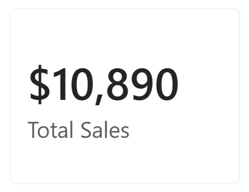
Total Sales = SUM(Sales[Amount])

When placed on a card visual, the measure returns the grand total across all visible data.

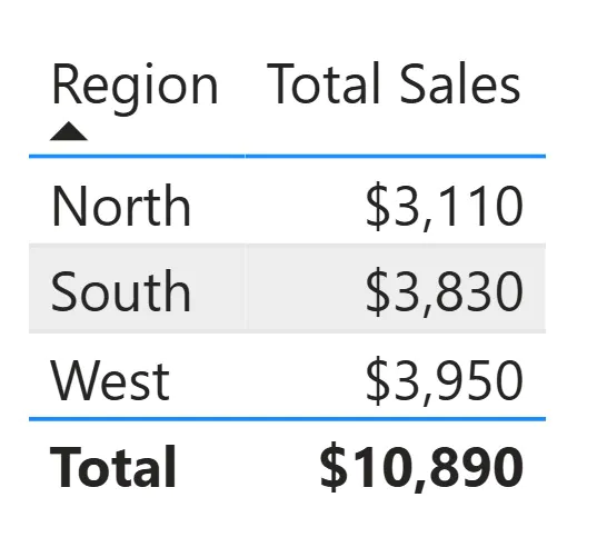
When placed in a table with Region on the rows, the same measure returns a different value for each row.

Each row applies a filter such as “Region equals North” before the measure evaluates.

Adding a Year slicer applies another filter layer on top. Every number adjusts accordingly.

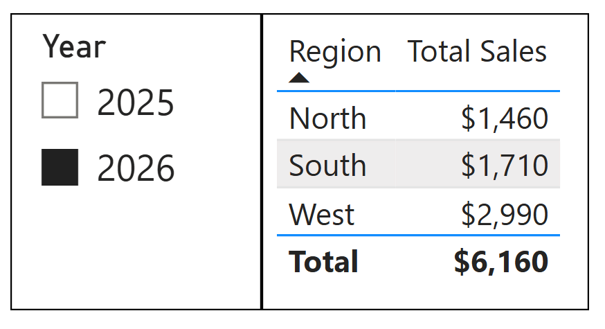
The measure logic remains unchanged. Only the filter context evolves.

How Filters Propagate Through the Data Model

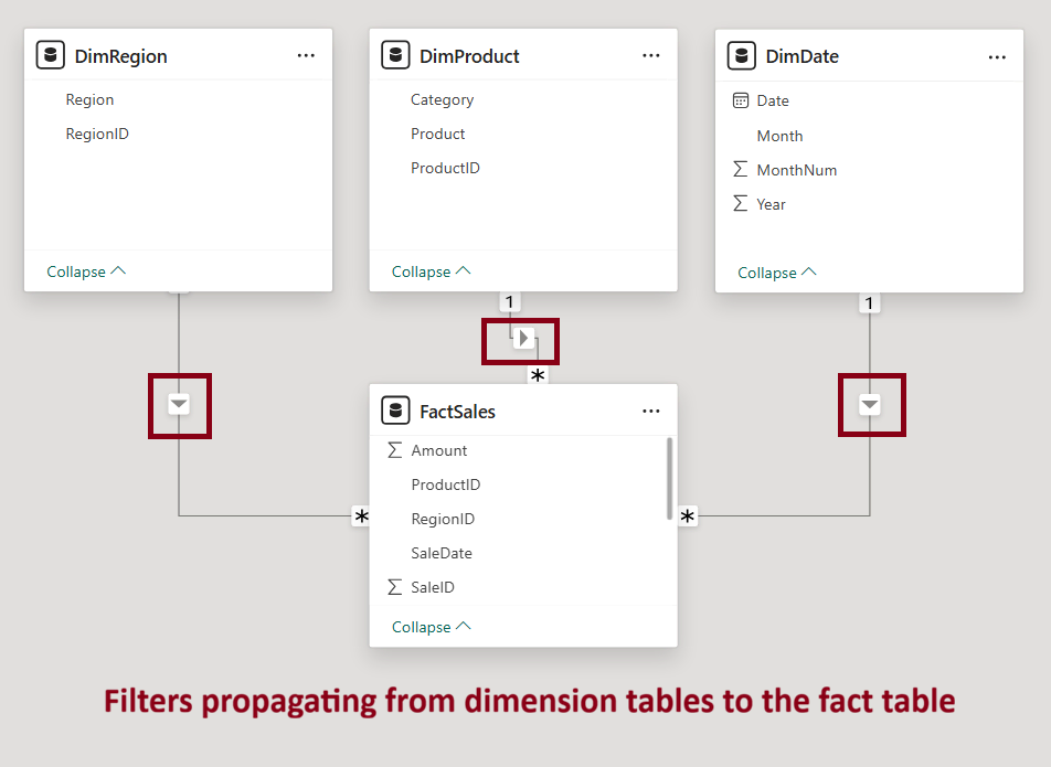
Filters do not stop at the table where they originate. They propagate through relationships in the model.

In a star schema, filters typically flow from dimension tables into fact tables. A slicer on a Product or Customer table filters the Sales fact table through the relationship.

This is why the star schema is recommended. It keeps filter propagation predictable and easy to reason about.

Confusion often arises in more complex setups, including:

• Bidirectional relationships
• Many-to-many relationships
• Inactive relationships

Bidirectional filters can cause filters to flow in both ways between tables. This sounds useful, but it creates ambiguity and can produce numbers that seem correct but aren’t.

Unless you have a very specific reason for it, keep your relationships single-direction (dimension → fact).

Context Transition and CALCULATE (The Turning Point)

Understanding that filter context exists is only the first step. Control over filter context is what turns confusion into intention.

That control is provided by CALCULATE.

CALCULATE evaluates an expression inside a modified filter context. Filters can be added, removed, or overridden before the expression runs.

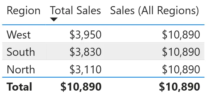
Sales (All Regions) =
CALCULATE(SUM(Sales[Amount]),
REMOVEFILTERS(DimRegion[Region]))

This measure ignores any Region filters and always returns the company-wide total as you can see below.

According to Microsoft’s CALCULATE documentation, CALCULATE is the only DAX function capable of modifying filter context. All other functions evaluate within whatever context already exists.

Removing, Keeping, and Overriding Filters

A few functions are used frequently to manage filter behaviour. Here are some of the most common:

• ALL and REMOVEFILTERS to ignore filters
• ALLEXCEPT to keep specific filters and remove others
• KEEPFILTERS to add filters without overwriting existing ones

ALLEXCEPT example

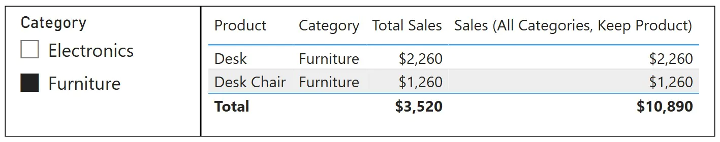
A table shows sales by Product, with a Category slicer present. Category selections should be ignored while Product row context is preserved.

Sales (All Categories, Keep Product) =
CALCULATE(SUM(FactSales[Amount]),
ALLEXCEPT(DimProduct, DimProduct[Product]))

Category slicer selections no longer influence the result, while each Product row continues to evaluate independently.

In this example, Total Sales responds to the category slicer, whereas the ALLEXCEPT measure ignores it and returns total sales regardless of the selected category.

KEEPFILTERS example

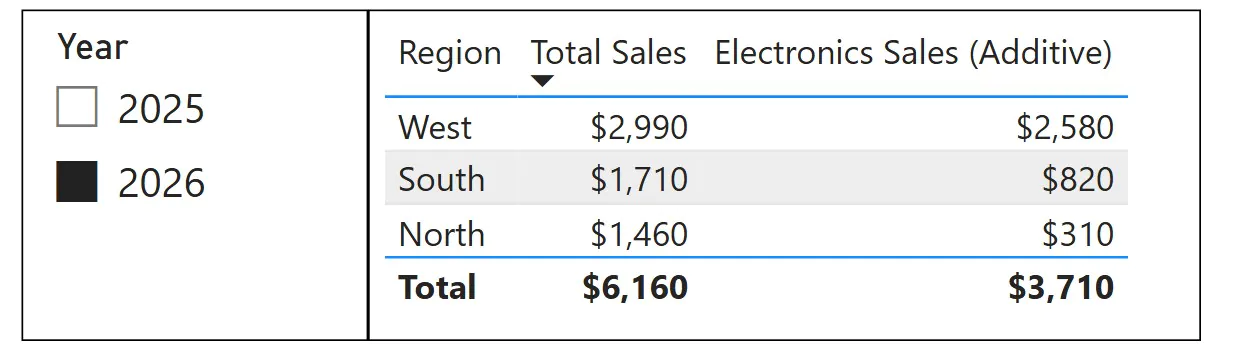
Electronics sales should always be shown, while still respecting Region and Year slicers.

Electronics Sales (Additive) =
CALCULATE(SUM(FactSales[Amount]),
KEEPFILTERS(DimProduct[Category] = “Electronics”))

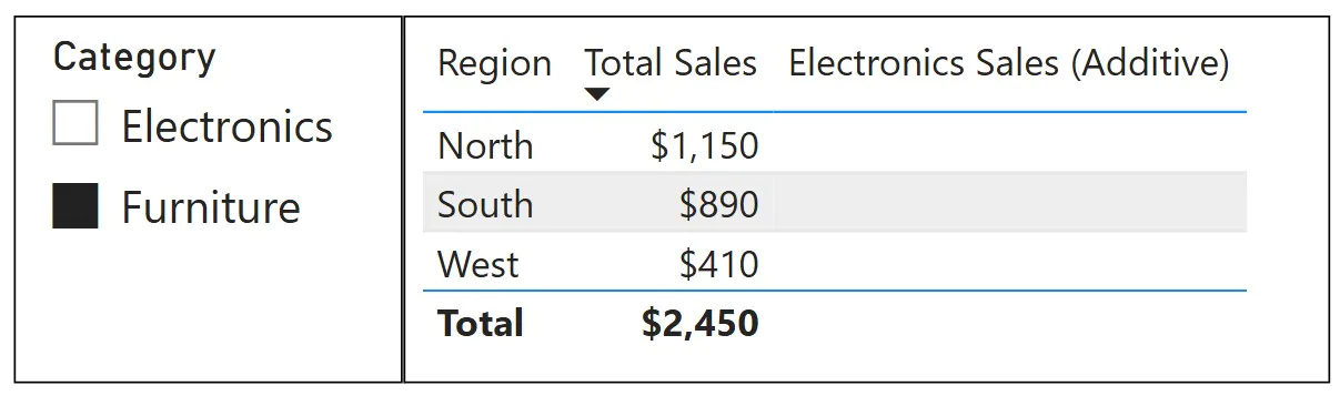
With KEEPFILTERS, filters are intersected rather than overwritten. When slicer selections conflict, the result is blank, which is the expected behaviour.

In this example, the Year slicer is still respected, but selecting Furniture in the Category slicer causes the measure to return blank.

ALL Example

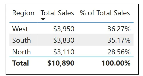
Percent of total calculations rely directly on filter context control.

% of Total Sales =
DIVIDE(SUM(Sales[Amount]),
CALCULATE(SUM(Sales[Amount]), ALL(Sales)))

The numerator respects the current context. The denominator removes it. The result is a correct percentage per row.

Debugging Filter Context When Numbers Look Wrong

Unexpected numbers are usually context problems, not math problems.

A reliable debugging workflow includes:

1. Recreate the visual output in a table with the same dimensions
2. Add slicers one at a time and observe where values change
3. Create temporary helper measures such as:
   Selected Region = SELECTEDVALUE(DimRegion[Region], “Multiple or None”)
4. Check relationship directions and cardinality

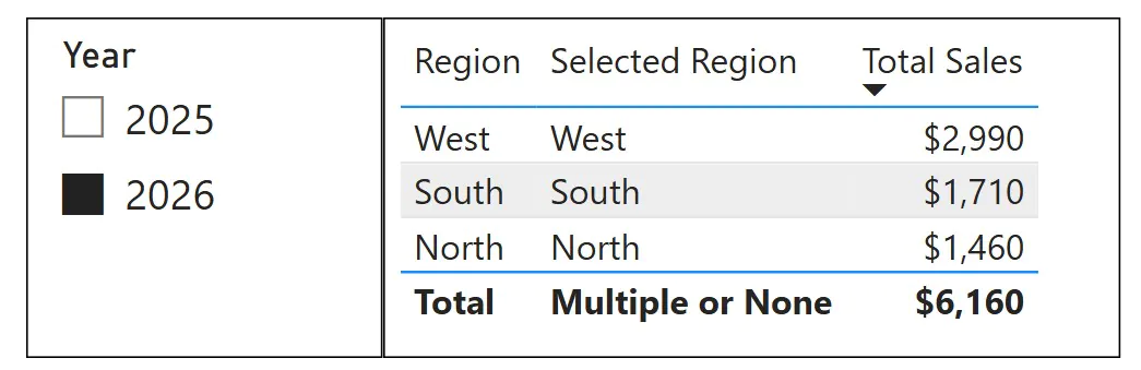
In this example, the helper measure confirms the active filter context for each row.

SELECTEDVALUE returns the region name when a single region is in context and falls back to the default when multiple regions or no region is selected. This makes it easier to verify exactly which filters each row is evaluating under when totals appear incorrect.

Common mistakes include relying on SELECTEDVALUE without handling blanks, and using ALL when only slicer selections should be ignored.

Best Practices for Predictable Measures

So if you want your practices to be predictable, what can you do?

We recommend you keep these 5 principles in mind:

• Be explicit about which filters a measure respects or ignores
• Try to build readable measures over clever ones
• Name measures based on their context assumptions
• Treat bidirectional and many-to-many relationships as advanced tools
• Test performance with Performance Analyzer when context logic becomes complex

Limitations and Edge Cases

Filter context becomes harder to reason about in scenarios involving:

• Many-to-many relationships
• Composite models and DirectQuery
• Calculation groups
• Ambiguous relationship paths

When possible, simpler models with well-defined relationships reduce risk and improve predictability.

The Iterator Trap: Row And Filter Context

There’s one last common trap we wrap up: context transition. This one that really trips people up, we have spent a lot of time in our Power BI advanced workshops finding the best way to explain it!

When an iterator function (think SUMX, AVERAGEX, MAXX) moves through each row of a table, it creates row context. The transition happens when a measure is called inside that iterator – at that moment, DAX automatically takes the current row context into its equivalent filter context with CALCULATE.

Sounds confusing, so let’s simplify down a bit. Say you have a measure that calculates average order value:

AvgOrderValue = AVERAGEX(Sales, Sales[Quantity] * Sales[Unit Price])

This works correctly, because it’s multiplying column values – it’s staying in its row context.

Now imagine the expression inside SUMX references another measure, rather than a column.

Total Margin = SUMX(Sales, [Gross Profit Measure])

Because [Gross Profit Measure] is a measure, not a column, calling it inside SUMX triggers context transition. The current row’s values become filter context, and the measure evaluates in that context. Often this is used intentionally, but it can produce results that seem incorrect if the measure uses functions like ALL that rely on context.

Our Advice: Be very cautious when calling measures inside iterators. If a SUMX or AVERAGEX is producing unexpected totals, check if it references a measure. If it does, try replacing it with an underlying column expression and see if the result changes.