SUMIFS for Budget Reporting: Build A Summary Dashboard Without Pivot Tables

We run Excel workshops in London every month, so we get to spot a lot of trends on how users use Excel at their jobs.

There are countless project managers and finance assistants all over the UK building summary dashboards, all doing the same thing.

They open their raw spend data, build a pivot table, drag a few fields around, get a summary that roughly looks right – then spend the next twenty minutes reformatting it before they can send it anywhere.

Sometimes the columns have shifted, the totals row isn’t showing up, or the colour coding they used last month is gone.

This is not a pivot table problem, pivot tables are excellent tools! The issue is using them for the wrong job.

If you need to explore data – rotating it, slicing it, asking “what does this look like by region?” – pivot tables are unbeatable.

But if you just need a report that always looks the same, month after month, we really recommend SUMIFS.

SUMIFS Function Syntax

The SUMIFS function adds up values in a range just like the SUM Function, but only for rows that meet multiple conditions at once.

The structure looks like this:

=SUMIFS(sum_range, criteria_range1, criteria1, [criteria_range2, criteria2], …)

• sum_range – the column containing the numbers you want to add up
• criteria_range1 – the first column to check against a condition
• criteria1 – the condition to apply to that column
• Additional criteria range/criteria pairs can be added as needed (you can add up to 127!)

Every condition must be true at the same time for a row to be included. That AND logic is key and cannot be changed.

Simple Example – Total Spend For One Department

We’ll build up slowly from the ground up, so let’s just start with using one condition for SUMIFS.

Imagine you’re working in a finance team, tracking project expenditure across departments.

Here’s the sample data:

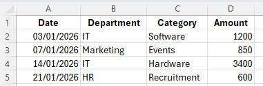
It’s a transaction log – with columns for date, department, category, and amount. You want to pull the total spend for the IT department.

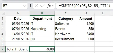
Type the following formula to get total IT spend:

=SUMIFS(D2:D5,B2:B5,”IT”)

• D:D is the Amount column – the numbers we want to sum
• B:B is the Department column – where to check the condition
• “IT” is the condition to match – as we just want to look at IT

And just like that, you get the total for IT only. Any row where the Department column says something other than “IT” is ignored completely.

That’s how you use SUMIFS at a basic level – just one condition. Let’s take a look at how you can start building on top of this foundation.

Advanced Example – Budget Summary By Department and Month

This is the scenario most people actually need, and it’s where SUMIFS separates itself from a basic filter or a pivot table.

Let’s say your director wants a fixed monthly report showing spend by department, broken down by month, with a variance against budget.

The report needs to look identical every single month – same rows, same columns, same formatting – because it goes into a board pack.

This is going to be a practical workflow, so this time we will format our data as a table and set up a summary table:

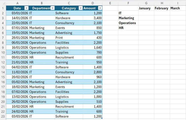
And then we will write a SUMIFS formula to populate each cell. For IT spend in January:

=SUMIFS(Table1[Amount], Table1[Department], “IT”, Table1[Date], “>=”&DATE(2026,1,1), Table1[Date], “<=”&DATE(2026,1,31))

Breaking that down piece by piece:

• Table1[Amount] – sum the Amount column on your Data table
• Table1[Department], “IT” – check the Department column and only include rows where Department is IT
• “>=”&DATE(2026,1,1) – only include rows where the date is on or after 1 January
• “<=”&DATE(2026,1,31)– only include rows where the date is on or before 31 January

Three conditions, all of which must be true at once.

From here, we can copy the formula, adjusting the date and department for each. 

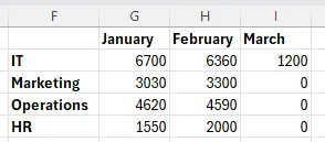
This is the key difference from a pivot table. You can design the layout, and SUMIFS will fill it in.

The layout never changes, regardless of what happens to the underlying data.

When You Should Still Use a Pivot Table

A core skill that makes a productive and efficient Excel user is picking the right tools.

On its initial release and when lots of us learned Excel, it had a much simpler tool set, and there was always one tool that was right for the job. Modern Excel on the other hand, has loads of options for each task – all with their own pros and cons.

When it’s time for you to produce something like our budget summary, don’t dive straight in and start building it. Take a moment to think about what you are making, and what tool will work best for you.

Pivot tables are great for Accounting & Bookkeeping, they’re ideal when you are exploring data, and need to analyse or reorganise your dataset. The drawback is that they only calculate when refreshed.

In our example, either tool would work, but SUMIFS will update whenever your dataset changes – and are generally just quicker to write. These are the things you want to think about when picking the right tool for the job.

It’s not a simple case of always using SUMIFS instead of Pivot Tables. Most experienced Excel users use both: pivot tables for exploration, SUMIFS for production reporting. 

Conclusion

SUMIFS is a simple function to understand and use, but powerful because of the conditional logic it uses. 

The way it uses multiple conditions is not just easy to write, but also easy for your colleagues to understand and trace through.

When it comes to monthly reporting, rebuilding and reformatting a pivot table every time is going to waste a lot of time!

Use this guide as an example, all you have to do is build the summary table once, write the formulas once, and let SUMIFS do the work.