Building A Solid Data Cleaning Architecture: Guided Walkthrough

How does an Excel pro in 2026 turn messy data into a clean, reporting ready dataset?

They design a complete, repeatable system.

Modern Excel expertise isn’t just knowing formulas, it’s understanding how Excel works in the real world.

Importing messy data, structuring it properly, transforming it efficiently, and producing reliable outputs no matter what.

It’s not about fixing spreadsheets, it’s about building real world processes.

In this guide, we’ll walk through an example from our popular Excel workshops in the City of London, a complete walkthrough of cleaning a dataset.

Not as a one-off exercise, but as a repeatable system you can keep coming back to.

Download The Raw Dataset

Start by downloading the sample expense report here.

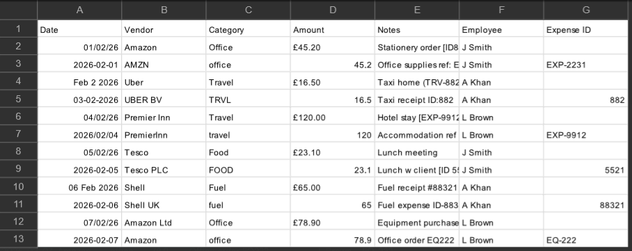
You’ll notice when you take a look, the file is full of inconsistent formatting, duplicate names, messy categories, numbers stored as text, important details hidden in notes, and missing values.

If you’ve used Excel in the working world, you won’t be too surprised!

Step 1 – Don’t Mess With The Raw File

Now, a lot of us will want to just open this file directly and start “fixing” the data. This is never the best move.

We want our process to be clear and repeatable for you and other people on your team, we don’t want step 1 to be something nobody can trace through. Never work directly on the export.

Instead, we will:

1. Leave the CSV alone
2. Create a working sheet in Excel
3. Perform the cleaning there

Your source data needs to remain a reliable source, if you edit it by hand then you’ll get lost information, and might end up breaking something later on when it’s too late. The workflow needs to be:

Raw Data → Transformation → Output

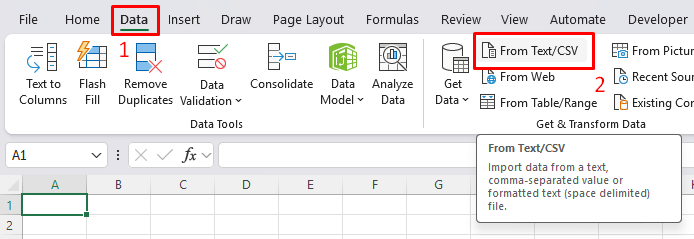
So let’s start off by importing out data into Excel, from the ribbon go to Data, then Get Data from CSV.

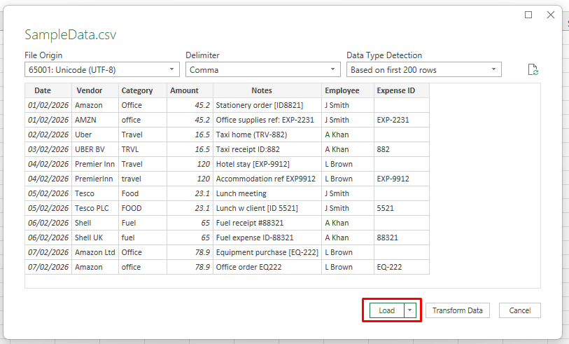
You’ll see a dialog box with your sample data, just go ahead and load it up as is.

Step 2 – Establishing And Enforcing A Clear Structure

Before we go ahead and adjust the values, we need to establish a clear structure.

This stage is all about planning, create a solid structure, and pay attention to places that aren’t following it.

We can make small changes here, like adjusting formatting, but we won’t apply any formulas or Power Query.

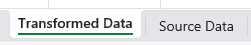
First things first, duplicate the sheet you are working with, so you can have the source and transformed data separately.

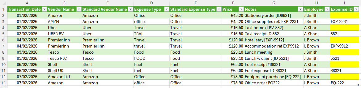
In Transformed Data, convert the data into a table, check the headers, and confirm column types.

For our data, I am going to rename some of the headers, as I want them to be more informative.

I’m also going to highlight the missing values in yellow, so I know to come back and fix them later.

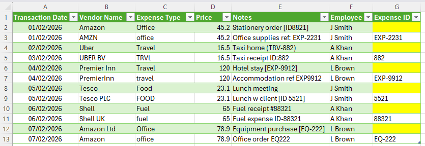
If we click around on the table, we’ll see that the date column has been picked up by Excel, and is in the correct date format.

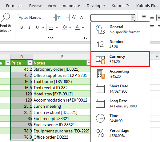
However, other fields, like the price, aren’t being formatted as a currency correctly.

Select all the data in the price column, and then convert it to a currency.

Step 3 – Picking Your Cleaning Tool

Typically, an Excel user will default to using formulas to clean up their data.

But modern Excel has all sorts of powerful features, so we’ll split data cleaning into two main options – Formulas and Power Query.

For this guide, we’ll show you how to implement both options so you get some experience, and can pick the approach you like best in future.

Formulas are often the fastest way to dive straight in, you can pick one problem and start testing things to fix it. You work directly in the sheet, and see results update instantly as you change things. If you’re dealing with a smaller dataset, or you need to dig around to actually figure out what’s wrong with the data – then we recommend starting with formulas. They’re flexible, visible, and easy to adjust as you keep building on it. A lot of teams will prefer to work with formulas as they can easily go and see the logic that you have used.

Power Query approaches the same problem from a different angle. Instead of fixing values directly in the sheet, you record a sequence of repeatable transformation steps that you can replay whenever new data rolls in. It is extremely powerful for repeatable workflows. If you receive the same type of report every week, Power Query can let you clean it once, and rerun the process next time. It also tends to handle larger datasets more comfortably than formulas, and keeps your cleaning logic separate from your final reporting sheet.

In practice, Excel pros don’t really rely on just one tool exclusively. They use formulas to explore and test things, then use Power Query to standardise and automate those conclusions. We aren’t trying to pick between two separate paths, we’re trying to understand how the tools work and work together to get a reliable and efficient result.

Step 4 – Cleaning With Formulas

Let’s get started with formulas.

The Vendor Column

Our first problem is the Vendor column, it has several entries that are similar, but with different names – for example we have Amazon, AMZN and Amazon Ltd.

While this is fine on a surface level, if you want to analyse this data later down the line with a PivotTable, you’ll get multiple entries for the same supplier.

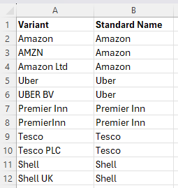
Instead of manually editing them, we are going to build a small mapping table. On a new sheet called Standard Names, create two columns: Variant and Standard Name.

The Variant column needs to include every variation in your data, then pick a standard name.

You can either do this logically yourself, or agree a set of standard names with your colleagues.

Now back to your Transformed Data sheet, insert a new column alongside Vendor Name, and in the first cell:

=XLOOKUP([@[Vendor Name]],’Standard Names’!A:A,’Standard Names’!B:B,[@[Vendor Name]])

The formula will automatically fill down to the rest of the cells:

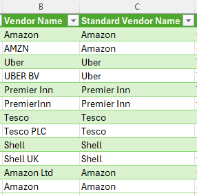
Now, the reason we used a mapping table is that in future, more and more variants are going to crop up. With our table, all you have to do is update it with new occurrences.

Since your XLOOKUP references the table, it will automatically update when you change the mapping table.

The Expense Types

Now, if you look at the Category column, you’ll see a very similar issue. We have Travel, TRVL and travel.

Try this one on your own! It’s a great test exercise, and will help you build the way you approach and think about these problems.

Here, you need to follow a simple plan. Decide Standard Names → Create A Mapping Table  → Reference The Names.

For a quick tip, you can use the same sheet (Standard Names)

You should be left with something like this:

Step 5 – Implementing Regex

These were pretty simple fixes, but it’s not always going to be easy! Looking at the Expense ID, we can see some of the IDs are there, but the formatting is inconsistent, and they aren’t all there.

In the Notes column, we can see more of the IDs, that are buried somewhere they shouldn’t be. Our next challenge is going to be extracting it.

This is where modern Excel pros are going to use REGEXEXTRACT.

Our full guide to regex and REGEXEXTRACT is here, but for our purposes – it uses its own language to let you define the pattern of what you’re looking for. Older text functions in Excel rely on exact positions, or stacking up several functions to get what you need.

For our example here, we just want to pull out the numbers from the notes tab.

Make a new “Standard Expense ID” column and type:

=IFERROR(REGEXEXTRACT([@Notes],”\d+”),”No ID”)

This uses regex to pull out \d+. The \d means any number, and the + means one or more digits.

We also wrap it with an IFERROR, which returns “No ID” if we don’t find one.

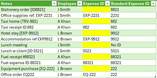
And just like that, our data is clean!

Step 6 – Cleaning With Power Query

We cleaned up our data pretty efficiently and quickly, but you don’t want to be redoing this week after week.

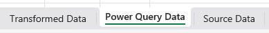
This is where Power Query becomes a much more obvious choice. Start out by duplicating your Source Data again, and putting it in a new sheet, “Power Query Data”.

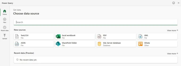
Then select your table, and go to Data → From Table/Range

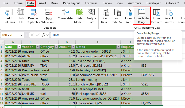
And you’ll see the Power Query editor. Might seem intimidating but we’ll take it slow!

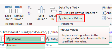
First, to replicate what we did with the Vendor Column, click on the Vendor column so it gets highlighted in Green, then click Replace Values.

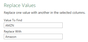
Here, you need to go through and type the value you currently have, and what you want it to be, so use the mapping table we made before!

Type in each variant one by one, and the standard names – do this for the Vendor and Category as before.

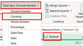
Then, to mimic what we did to the currencies, click the Currency column and change it with the Data Type.

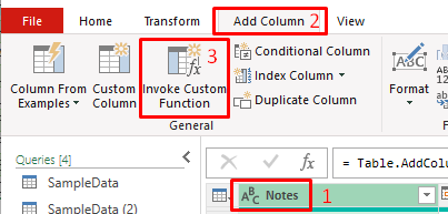
Finally, we need to extract those numbers from the Notes column. Now we used regex before, but Power Query has its own way!

Click the Notes column, then go to Add Column, and Invoke Custom Function.

Then just type in this formula:

=Text.Select([Notes], {“0”..”9″})

This will pull out the numbers from the notes column, similar to the regex we used before.

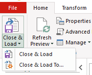
Now our data is all tidied up again! Just click Close & Load, and your data will flow into Excel.

Now the magic here comes from the reusability.

Power Query has saved all the steps you’ve made, replacing values, changing formats, and extracting data.

Now when you adjust the data in the Power Query Data tab, you can hit the refresh button to rerun the same Power Query process on it.

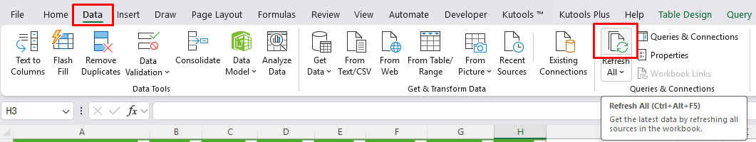
The same steps will be run through again, and suddenly your data set is being cleaned automatically.

Step 7 – Building A Repeatable Workflow

So now our data has been cleaned in two different ways.

We’ve used formulas to experiment and fix issues in the sheet, and used Power Query to apply transformations in a structured, repeatable way. Now it’s time to think about the process instead of the cleaning itself.

An Excel pro isn’t trying to just fix one dataset. They know what kind of data they are working with each week, and who else on the team needs to use it.

At this stage, your process should look something like this:

Raw CSV → Import To Excel → Transform → Output For Reporting

When a new expense export arrives, you don’t want to start again from scratch. You want to drop the data into the same place, refresh Power Query, and your dataset updates automatically.

The formulas and functions you used helped you understand your data, and what you want from it – but it needs to be finalised in Power Query.

Conclusion

Excel proficiency in 2026 isn’t about knowing as many formulas as possible.

It’s about understanding how Excel fits into real work, importing data properly, structuring it clearly, and choosing the right tools to transform it.

In this walkthrough, we cleaned a dataset, but also built a process at the same time.

We used formulas to explore and standardise, regex to extract patterns, and Power Query to create a repeatable transformation.

Each step had it’s own purpose, and together they formed a complete workflow that can be reused whenever new data arrives.

That’s how Excel pros work.