Excel’s GROUPBY Function: What It Does & When to Use It

If you’ve ever built a summary table in Excel by writing five separate SUMIFS formulas – one for each region, product, or department – you’ll appreciate what GROUPBY does.

It collapses all of that into a single formula that updates automatically, sorts itself, and can even filter out rows you don’t care about.

Introduced to Microsoft 365 in late 2024, GROUPBY is one of the most practically useful additions Excel has had in years.

But it also comes with real limitations that most people gloss over.

What Does GROUPBY Actually Do?

GROUPBY summarises data by grouping rows that share a common value and running a calculation on them – a sum, average, count, maximum, or any other aggregation you choose.

The result spills into a dynamic range automatically, just like FILTER or UNIQUE.

Here’s the simplest way to think about it: you’re telling Excel “group my data by column A, add up column B, and show me the results.”

What you get back looks like a one-column pivot table – but written as a formula.

The syntax is:

• row_fields – the column(s) you want to group by (e.g. Region, Product)
• values – the column containing the numbers to aggregate
• function – SUM, AVERAGE, COUNT, COUNTA, MAX, MIN, etc.
• field_headers – whether to show column headers in the output
• total_depth – whether to add grand totals or subtotals
• sort_order – which column to sort by, and in which direction
• filter_array – a logical expression to exclude certain rows
• field_relationship – how multiple row_field columns relate to each other (hierarchy or flat)

A Real Example: Sales by Region (In Stages!)

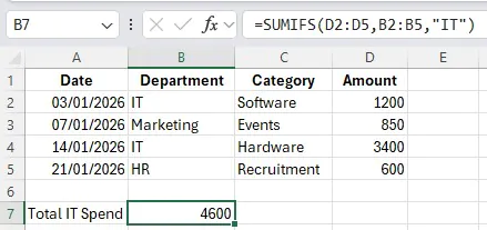
Imagine you work in a sales operations role, and you want a quick breakdown of total revenue by region. Your data has three columns: Salesperson, Region, and Revenue.

Instead of writing:

=SUMIF(B2:B16, “North”, C2:C16)

…and then repeating it for South, East, and West – you write one formula:

=GROUPBY(B2:B2, C2:C16, SUM)

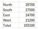
Excel returns a two-column table: each unique region in the left column, its total revenue on the right.

If a new region appears in your data tomorrow, it appears in the output automatically.

GROUPBY is a pretty big and complex formula, we find on our Excel training workshops in London that the best way to learn it is piece by piece.

So stick around for how you can adapt the formula with its huge list of arguments!

Sorting the Results

By default, GROUPBY sorts alphabetically by the row field. If you want to sort by value instead – say, the highest revenue at the top – use the sort_order argument.

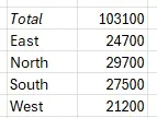
To sort by the second column (revenue) in descending order:

=GROUPBY(B2:B16, C2:C16, SUM, , , -2)

The negative number means descending. A positive number (e.g. 2) means ascending. The number refers to the column position in the output, not in your source data.

This is something that trips people up in training. The sort_order argument looks deceptively simple, but the column numbering refers to the output table, not the input range.

If you’re grouping by two fields, the values’ column might be column 3, not column 2.

Adding Grand Totals

The total_depth argument controls whether totals appear:

0 – no totals
1 – grand total at the bottom
2 – grand total and subtotals (useful when grouping by multiple fields)
-1 – grand total at the top

So using =GROUPBY(B2:B16, C2:C16, SUM, , -1) gives you:

Filtering Within the Formula

One of GROUPBY’s underappreciated features is the filter_array argument. You can exclude rows without touching your source data.

Say you want totals by region, but only for sales over £5,000:

=GROUPBY(B2:B16, C2:C16, SUM, , , , C2:C16>5000)

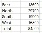
The filter argument takes a logical array – any expression that returns TRUE or FALSE for each row.

The Formatting Catch

Here’s something most guides don’t flag clearly enough: GROUPBY output cannot be formatted with Excel’s “Format as Table” feature.

Because it’s a dynamic array that spills, you can’t convert the output range to a structured table.

This means you have to apply number formatting, borders, and cell shading manually – and if the spill range grows (because new groups appear in your data), that formatting won’t extend automatically to new rows.

For polished reports that other people will read, this is a genuine drawback.

Pivot table formatting is more limited in some ways, but it at least scales with the data.

From Our Training Rooms

When we introduce GROUPBY to Excel students, the feature they like the most is usually the auto-refresh.

Pivot tables have tripped people up for years – you update the source data, the pivot table looks wrong, someone panics, and eventually someone remembers to right-click and refresh. GROUPBY removes that friction entirely.

The trickier adjustment is the mindset shift. Pivot tables are interactive: you drag fields, click filters, and experiment visually.

GROUPBY is declarative – you write exactly what you want in the formula, and that’s what you get.

Students who are comfortable with formulas tend to take to it quickly.

Those who prefer working visually often find pivot tables more intuitive for complex reporting, even once they understand what GROUPBY can do.

Neither approach is wrong. The best Excel users know which tool suits which situation.

Summary

GROUPBY is a genuinely useful addition to Excel – particularly for anyone building formula-driven workbooks where live, auto-refreshing summaries matter.

It’s cleaner than a bank of SUMIFS formulas and more consumable than a pivot table.

But it’s not a pivot table killer. For complex reporting, multi-aggregation views, large datasets, or outputs shared with non-technical colleagues, pivot tables remain the more practical and accessible choice.