Linking Data in MS Excel
What if all your data could be linked across from one sheet to another?
You would stop needing multiple copies of the same data.
You’d also minimize the risk of incorrect data due to forgetting to update the information across sheets!
It is an excellent way to make it very simple to create a summary of up to date data.
This becomes especially important when multiple people are working on the same spreadsheet.
Before we start, here is what a sheet of the source data in excel looks like:
Method 1 – Cell Formula Writing + Clicking
First, click the cell in the worksheet you want the data to appear in:
- Type in the formula bar “=”
- Click on the information in the source worksheet you want to carry across
- Press enter
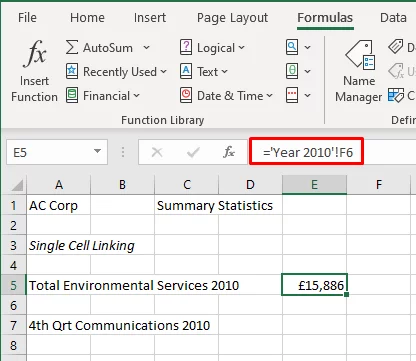
The formula bar will show where the information has been linked to, the sheet name, an exclamation mark and the cell number:
Note you can link to named ranges as well as cells.
Method 2 – Copy And Paste
Start on the source worksheet and copy the information you want to link
- Right click on the cell in the destination sheet and go to ‘Paste special’
- Click on the ‘Data link’ icon. Interestingly, if you are used to opening up the paste special box, the link data option doesn’t appear in it.
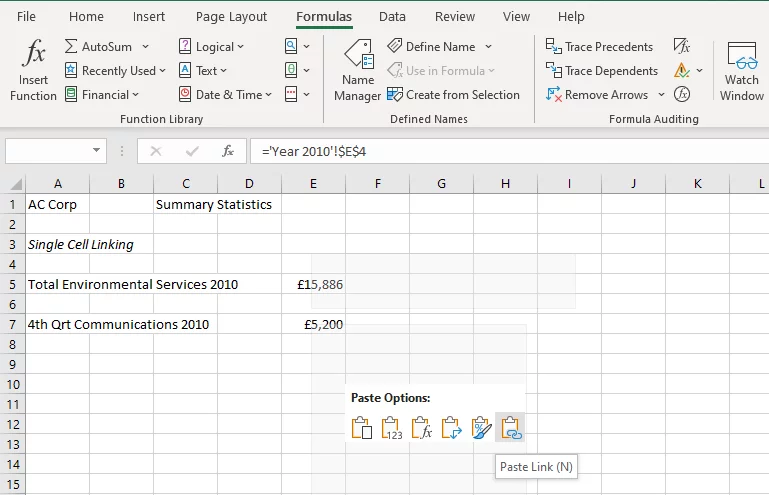
If you use this method, the cell is entered as an absolute cell reference.
You can learn about all types of cell references here.
Linking to Multiple Cells
You can also create a link to multiple sheets and cells to a single cell with a function.
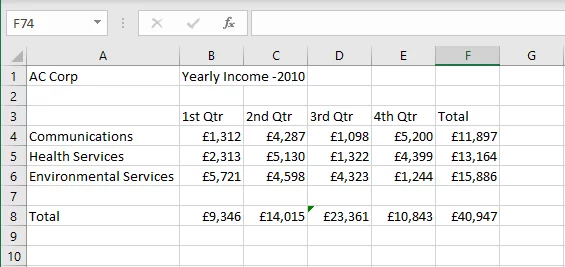
In the example below, the total spend on communications for three years has been shown on the summary sheet:
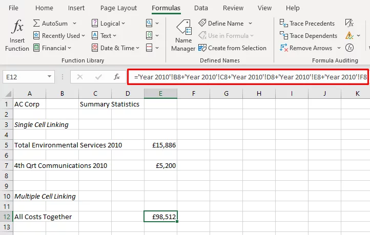
To do this, you will use method 1 above but after clicking on the first total in 2010, press ‘+’ then click the next piece of data and so on.
Excel offers lots of different ways to validate and track your data. Overtime you will work with larger, more complex spreadsheets ands o will need to be sure that your skills keep pace.